Imposing Functional Priors on Bayesian Neural Networks

Bogdan Kozyrskiy

, Dimitrios Milios

and Maurizio Filippone

Department of Data Science, EURECOM, 450 Route des Chappes, Biot, France

Jubile Tech Ltd., London, U.K.

Keywords:

Bayesian Inference, Markov Chain Monte-Carlo, Deep Neural Networks.

Abstract:

Specifying sensible priors for Bayesian neural networks (BNNs) is key to obtain state-of-the-art predictive

performance while obtaining sound predictive uncertainties. However, this is generally difﬁcult because of the

complex way prior distributions induce distributions over the functions that BNNs can represent. Switching

the focus from the prior over the weights to such functional priors allows for the reasoning on what meaningful

prior information should be incorporated. We propose to enforce such meaningful functional priors through

Gaussian processes (GPs), which we view as a form of implicit prior over the weights, and we employ scalable

Markov chain Monte Carlo (MCMC) to obtain samples from an approximation to the posterior distribution

over BNN weights. Unlike previous approaches, our proposal does not require the modiﬁcation of the original

BNN model, it does not require any expensive preliminary optimization, and it can use any inference tech-

niques and any functional prior that can be expressed in closed form. We illustrate the effectiveness of our

approach with an extensive experimental campaign.

1 INTRODUCTION

Artiﬁcial Neural Networks (NN) currently represent

a general class of successful models for various ma-

chine learning tasks, including computer vision, nat-

ural language processing, and many others. Bayesian

Neural Networks (BNN) combine the representation

power of NNs with Bayesian inference, making them

an attractive choice in applications where predictive

performance and accurate uncertainty quantiﬁcation

is important. BNNs are difﬁcult to use because of

the intractability of the posterior over model param-

eters, which necessitates approximations. Choosing

appropriate priors over model parameters is also cru-

cial for good performance (Fortuin, 2022; Tran et al.,

2022). In BNNs, the prior over the weights and the

network architecture determine a distribution over the

outputs of such BNNs (Sun et al., 2019), and we re-

fer to this induced prior as a functional prior. The

functional prior should encode any prior information

on the conditional distribution of the labels given the

inputs. However, it is unclear how to encode this type

of information when having to specify a prior distri-

bution over the weights.

This paper presents a framework for imposing

meaningful functional priors using scalable Markov

chain Monte Carlo (MCMC) sampling from an ap-

proximation to the posterior distribution over BNN

weights, and we specify the prior over the weights

implicitly through a prior over the induced functional

prior. Our approach is different from the literature

on Implicit Process Priors (IPPs) (Ma et al., 2019),

where the goal is to obtain an approximate frame-

work to handle the functional prior implicitly induced

by the choice of a prior distribution over the weights.

In our work, we operate in the opposite direction by

imposing a functional prior, which implicitly deter-

mines a prior over the weights; we do not know such

a prior over the weights in closed form, but we im-

plicitly determine it through the speciﬁcation of the

induced functional prior.

Stochastic Processes are natural mathematical ob-

jects suitable to deﬁne distributions over functions

(Kallenberg and Kallenberg, 1997), and Gaussian

Processes (GPs) represent popular examples which

are routinely used in numerous machine learning

tasks. This type of stochastic processes is well

investigated and has strong theoretical foundations

(Williams and Rasmussen, 2006). There are theo-

retical guarantees for the generalization error of GP

regression, and this method has a strong connection

with non-Bayesian Kernel Ridge Regression (KRRs)

(Kanagawa et al., 2018). Also, it was shown in (Neal,

1996) that in the inﬁnite width limit, shallow BNNs

are equivalent to GPs. We propose to use GPs to im-

pose functional priors over BNNs because GPs pro-

vide a ﬂexible set of tools to encode different types of

beliefs about functions, such as periodicity or smooth-

450

Kozyrskiy, B., Milios, D. and Filippone, M.

Imposing Functional Priors on Bayesian Neural Networks.

DOI: 10.5220/0011742900003411

In Proceedings of the 12th International Conference on Pattern Recognition Applications and Methods (ICPRAM 2023), pages 450-457

ISBN: 978-989-758-626-2; ISSN: 2184-4313

 2023 by SCITEPRESS – Science and Technology Publications, Lda. Under CC license (CC BY-NC-ND 4.0)

ness through the speciﬁcation of kernels. However,

our approach is not restricted to GPs, and it can han-

dle any functional priors that can be written down in

closed form.

This paper is organized as follows. We review the

related literature in Sec. 2, and we present our method

in Sec. 3. We report results on various benchmarks

in Sec. 4 and we conclude the paper in Sec. 6, after

discussing the limitations of our work in Sec. 5.

2 RELATED WORK

A popular way of choosing prior distributions for

BNNs is to employ a Gaussian distribution over the

weight of the model (Graves, 2011; Neal, 1996). This

offers some practical advantages, for instance when

employing Variational Inference (VI) (Graves, 2011).

Mean-ﬁeld VI allows for efﬁcient calculations of the

regularization part of the VI objective function with-

out the need to resort to Monte Carlo approximations,

but the limited ﬂexibility of the approximating distri-

butions may negatively affect performance.

Even when adopting more advanced and generally

more accurate inference techniques, such as Stochas-

tic Gradient Hamiltonian Monte Carlo (SG-HMC)

(Chen et al., 2014), the Gaussian assumption on the

prior over model parameters is still common. It was

shown by (Fortuin et al., 2021) that Gaussian priors

are problematic in terms of model performance and

the ability to detect Out-of-Domain (OOD) input ex-

amples. This work also shows how Gaussian priors

over the weights could be responsible for the cold

posterior effect described by (Wenzel et al., 2020);

this effect is characterized by the necessity of apply-

ing temperature scaling to the prior density term in

Bayes theorem in order to obtain good performance.

Flexible alternatives to Gaussian priors, such as

mixture of Gaussians (Blundell et al., 2015), Stu-

dent’s t-distribution (Fortuin et al., 2021), hierarchi-

cal Gaussian distribution (Chen et al., 2014) and many

others (Fortuin, 2022) were developed to address poor

performance of Gaussian priors. However, all these

types of priors still do not help understanding their

effect on model outputs.

An alternative to studying weight priors is to fo-

cus on their effect on NNs functional priors. A vari-

ational objective computed on a ﬁnite set of func-

tion evaluations is proposed in (Sun et al., 2019) for

ﬁnding a Bayesian posterior in the space of functions

for a functional prior deﬁned by a stochastic process.

The authors show that the supremum of the KL di-

vergence over all sets of input points is equal to the

true KL divergence in functional space. In this set-

ting, the optimization procedure simultaneously min-

imizes the optimization objective with respect to the

parameters of the model and maximizes the KL term

with respect to the input data points, which makes the

optimization process unstable. Also, the optimization

objective requires evaluating the gradient of the ap-

proximate posterior density by the Stein gradient es-

timator (Shi et al., 2018), and this requires a careful

choice of a kernel function. The work in (Ma et al.,

2019) focuses on representing the functional prior as

a BNN and uses GPs to obtain an approximate poste-

rior over functions. The problem with this approach

is that GPs may yield a poor approximation quality

for the true functional posterior. The authors in (Sun

et al., 2019) and (Ma et al., 2019) use VI to ﬁnd an

approximate posterior distribution, which means that

the optimization objective contains a functional KL

divergence term. However, in (Rudner et al., 2021) it

is claimed that the KL divergence between the func-

tional approximate posterior and the GP process func-

tional prior is problematic as it may diverge to inﬁn-

ity. On the other hand, they acknowledge that it does

not mean that parametric models cannot approximate

GPs well.

The authors of (Tran et al., 2022) propose to im-

pose functional GP priors so as to constrain the para-

metric prior over the weights of BNNs. They propose

to optimize parameters of the prior over the weights

by minimizing the Wasserstein distance between the

BNN functional prior and the GP prior. Then, the pos-

terior over the weights is characterized by means of

MCMC.

In our work, we aim to avoid the computation of

the KL divergence or any other distance metric in

function spaces. Instead, we propose to enforce the

choice of a functional prior directly when carrying out

approximate inference of BNN weights.

3 METHODS

Consider a supervised learning task with a dataset

D{(x

, y

)}

i=1...n

of n input vectors X =

{

}

i=1...,n

and corresponding labels y =

{

}

i=1...,n

, and imag-

ine employing a NN-based model with param-

eters w to establish a parametric mapping be-

tween inputs and labels. We denote the in-

put/output mapping by f

(x), and for convenience

we also deﬁne f

⊤

= [ f

), . . . , f

)] and f

∗⊤

[ f

), . . . , f

), f

(

), . . . , f

(

)] as the evalu-

ation of the function f

(x) at the inputs X and an aug-

mented set of inputs X

∗

= [X,

X], respectively. The set

∗

has cardinality N

∗

= N +

N, and the

N inputs in

are drawn from a given p(x). Note that the sets X and

Imposing Functional Priors on Bayesian Neural Networks

451

∗

can be disjoint, but in order to keep the notation

uncluttered, we assume X ⊂ X

∗

3.1 Imposing Functional Priors on

BNNs

A Bayesian treatment NNs requires specifying a prior

distribution p(w) over the parameters and a likeli-

hood function for the labels given the inputs, that is

p(y|X, w). For this BNN, it is possible to write down

an expression for the posterior distribution over model

parameters as:

p(w|y, X) =

p(y|X, w)p(w)

p(y|X, w)p(w)dw

(1)

Carrying out inference in BNNs is extremely dif-

ﬁcult for at least two reasons. One main difﬁculty

stems from the complex way in which parameters

affect the likelihood function, and this requires ap-

proximation techniques to characterize the posterior

over model parameters; popular approaches involve

MCMC and variational approximations. A second

and more subtle challenge is how to specify priors

for BNNs, because it is difﬁcult to establish what

is the effect of prior parameters on the distribution

over the functions that BNNs can represent. In this

work, we propose a novel way to address the chal-

lenge of choosing sensible priors for BNNs by work-

ing with implicit priors over the weights induced by

the choice of functional priors, while we follow the

recent trend to employ MCMC techniques to address

the intractability of the inference process. We begin

by focusing on the distribution over the functions rep-

resented by BNNs. In particular, we consider the dis-

tribution of f

∗

, which is the distribution of f

(x) eval-

uated at the set of input points X

∗

, and we impose a

prior over this set of variables which encourages func-

tions to behave in a sensible way a priori. Later we

will study in particular Gaussian process priors, but

any functional prior can be incorporated as long as it

can be expressed in closed form.

We now rewrite the likelihood function in terms of

f rather than w:

p(y|X, w) → p(y|f). (2)

The main idea behind our work is to now deﬁne a

prior over f instead of w, and to perform inference

over w. With this change of variables, we should ac-

count for the change of measure through a Jacobian

term. However, such a change of variables involves

groups of variables of different dimensions in general

and even when this is not the case, computing this

term would be computationally costly. For this rea-

son, we are going to ignore the Jacobian accepting to

settle for an approximate posterior over w. With this

choice, we rewrite Bayes theorem as:

log p(f

∗

|y, X

∗

) = log p(y|f) + log p(f

∗

) + const.

(3)

Note that in this equation we introduced the func-

tional prior:

p(f

∗

) =

p(f

∗

, w)p(w)dw, (4)

where p(f

∗

, w) is a Dirac’s delta placed at the eval-

uation of f

(x) at the inputs X

∗

due to the determin-

istic way in which inputs are mapped into outputs in

NNs. Again, we stress that while we focus on the dis-

tribution of functions represented by BNNs, we ac-

tually use the objective in eq. 3 to perform MCMC

sampling in the space of the weights w. Note that

we carry out inference over w through MCMC, but

given that we are working with an approximation to

the posterior over w, we could alternatively employ

other fast approximate inference techniques such as

VI. Here, we focus on MCMC so as to isolate the ef-

fect of the way we impose functional priors compared

with alternatives which try to characterize the exact

posterior over w (Tran et al., 2022).

Bayesian Interpretation. From a Bayesian point of

view, imposing a prior over function by specifying a

prior over f

∗

induces an implicit prior over the weights

through eq. 4. In other words, the prior over f

∗

is in

practice a prior over a deterministic transformation of

w, and this is implemented by the NN. It is interest-

ing to note that in the literature eq. 4 is usually in-

terpreted in the opposite way; that is, one uses eq. 4

starting from a prior over the weights p(w) to deﬁne

a functional prior in an implicit way (Ma et al., 2019).

The likelihood function establishes what is the like-

lihood of the labels y and it is conditioned on f or

equivalently on w and X. Therefore, the expression

in eq. 3 can be seen as an expression for the (approx-

imate) posterior over the weights w (due to the lack

of a Jacobian term), where the prior is assumed over

a transformation of such weights. In this paper, we

take this view to carry out Bayesian inference over

w using MCMC techniques. We also note that our

approach has some close similarity with the Product

of Expert approach proposed in (Wenk et al., 2019)

for inference of parameters of Ordinary Differential

Equations using Gaussian Processes.

Regularization Interpretation. While we proceed

with a Bayesian treatment of w, it is useful to interpret

eq. 3 as a regularized objective in the following way.

The ﬁrst term log p(y|f) is the negative loss, which

can be equivalently be seen as a function of w and

ICPRAM 2023 - 12th International Conference on Pattern Recognition Applications and Methods

452

∗

, so this provides a constraint on w because the

objective promotes values of f which are compatible

with the labels y, and f depends on w and X

∗

. The

second term is a regularization term, which penalizes

functions deviating from a behavior established by the

functional prior. Because f

∗

is a function of w and X

∗

this translates into a regularization term for w.

3.2 Imposing Functional Priors

Through Gaussian Processes

The proposed formulation focusing on functional rep-

resentations has the advantage of putting the empha-

sis on the functions that BNNs can represent, and for

which it is possible to assume sensible priors. Here

we specify how to operate in case of Gaussian pro-

cesses (GPs), which yield a prior term in eq. 3 as:

log p(f

∗

) = −

∗⊤

−1

∗

+ const, (5)

where the covariance matrix is C = (K

∗

+σ

), and

∗

contains the evaluation of the kernel function κ

among all the inputs in X

∗

. For simplicity, we assume

a zero-mean GP, but other mean functions can be eas-

ily included. In the next subsections, we elaborate on

how to use this GP prior in practice, by proposing a

way to operate with mini-batches for scalability pur-

poses, by discussing hyper-parameter optimization,

and by discussing the properties of the proposed ap-

proach when N

∗

goes to inﬁnity.

3.2.1 Mini-Batching

In this work, we aim to employ advanced MCMC

sampling methods based on stochastic gradients, and

in particular Stochastic Gradient Hamiltonian Monte

Carlo (SG-HMC) (Chen et al., 2014) to sample from

the weights w of BNNs. In order to do so, we need to

formulate our MCMC objective in a way that is suit-

able for mini-batching. However, extending the pre-

vious formulation to operate with mini-batches with-

out care would produce a biased estimation of the

quadratic term f

∗⊤

−1

∗

̸= E[f

∗⊤

−1

∗

], where f

and

are computed over a mini-batch X

The main difﬁculty of full batch training is the ne-

cessity of solving linear systems with the matrix C,

which has O(N

∗3

) complexity in the number of in-

puts in X

∗

. The literature on GPs offers many cues on

how to circumvent this problem. In particular, there

exist formulations of GPs based on random features

(Rahimi and Recht, 2007) which operate on mini-

batches (Cutajar et al., 2017). In this work, we fo-

cus on approximations based on random features, but

inducing points formulations are also possible.

Random Feature (RF) expansions of the kernel

κ(·, ·) allow one to obtain a ﬁnite-dimensional repre-

sentation for an explicit feature map which approx-

imates the true possibly inﬁnite-dimensional feature

map. Using this expansion, we can express the Gram

matrix as a dot product of feature maps computed

over the data K ≈ ΦΦ

⊤

. We can use this property and

the Woodbury identity to rewrite the quadratic term as

follows:

∗⊤

−1

∗

= f

∗⊤

(ΦΦ

⊤

+ σ

−1

∗

∗⊤

∗

−

∗⊤

Φ(Φ

⊤

Φ + σ

−1

⊤

∗

(6)

In this case, instead of inverting a matrix of size

∗

× N

∗

, we invert a matrix of size D × D, where

D is the dimensionality of the RF vector. However,

this approach has two drawbacks. First, it is unsta-

ble when σ

→ 0, because after the application of the

Woodbury identity the term

∗⊤

∗

→ ∞. Second,

this approach still does not allow mini-batching.

We can reformulate our MCMC objective by re-

placing the nonparametric term pertaining to the GP

with a parametric one based on RFs. For the set f

∗

we can factorize its prior probability as:

p(f

∗

) =

p(f

∗

|β, X

∗

)p(β)dβ, (7)

where β are the parameters of RF approximation of

the GP, that is p(β) ∼ N (0, I) and p(f

∗

|β, X

∗

) ∼

N (Φβ, σ

I). In this case it is easy to verify that

p(f

∗

) = N (0, ΦΦ

⊤

+σ

I) and according to the prop-

erty of the RF approximation, the covariance ma-

trix coincides with the prior term of the objective in

eq. 6. Instead of sampling directly from the unnormal-

ized posterior p(f

∗

, y) marginalized over β, we can

sample from the joint density p(f

∗

, β|X, y) and discard

samples over β:

p(f

∗

, β|X

∗

, y) ∝ p(y|f)p(f

∗

|β, X

∗

)p(β). (8)

Again, when we refer to the fact that we sample f

∗

in practice we sample w. This RF-based approach

avoids the necessity of inverting the matrix (ΦΦ

⊤

I) during the computation of the objective.

Resuming, the expression for the unnormalized

log-posterior in eq. 8, where the GP regularization is

approximated using RFs, is as follows:

log p(y|f) −

2σ

∥f

∗

− Φβ∥

−

||β||

+ const. (9)

It is straightforward to verify that this MCMC ob-

jective can be written as a sum of terms involving

individual input points, and it is therefore amenable

to mini-batching. It is also easy to verify that

Imposing Functional Priors on Bayesian Neural Networks

453

one can proceed with a Gibbs sampling scheme

whereby f

∗

(that is w) is sampled from the conditional

ˆp(f

∗

|β, X

∗

, y) using SG-HMC and β is sampled di-

rectly from ˆp(β|f

∗

, X

∗

, y), which has a Gaussian form.

3.2.2 Hyper-Parameter Optimization

The choice of a GP prior opens to the need to spec-

ify its kernel parameters. In the absence of any way

to determine such hyper-parameters, we propose to

optimize them by marginal log-likelihood (MLL) op-

timization, which is a popular way to proceed with

GP models. In our case, the random feature approxi-

mation lends itself to a scalable solution, avoiding the

need to invert large matrices. Again, using Woodbury

matrix identities, it is possible to rewrite the marginal

likelihood so that the cost of computing it is cubic in

the number of random features instead of cubic in the

number of input points.

3.2.3 Classiﬁcation

While for regression it is natural to specify func-

tional priors through GPs and to obtain a tractable

framework to scale these through random features, for

other likelihoods things may become more involved.

For instance, in classiﬁcation problems, we may wish

to specify functional priors such that the distribution

over classes is uniform a priori.

Alternatively, following an empirical Bayes ap-

proach, we could optimize the GP prior hyper-

parameters so as to maximize the marginal likeli-

hood. In this case, the random feature approximation

of GPs leads to so-called Generalized Linear Mod-

els (GLMs) and this requires approximations to be

able to compute the marginal likelihood. For classiﬁ-

cation tasks, there exist solutions to bypass the need

to work directly with Bernoulli or Multinoulli likeli-

hoods p(y|w, X). Here we follow the idea proposed

by (Milios et al., 2018), in which labels are trans-

formed so that classiﬁcation models can be replaced

by regression models with heteroskedastic observa-

tion noise. In particular, for each one-hot encoded

label y we can obtain real valued vectors

y, σ

(see

(Milios et al., 2018) for details):

˜y

= log(α

) −

;

= log



+ 1



. (10)

With this transformation, we can use a Gaussian like-

lihood which is conjugate to the Gaussian prior, and

thus we can obtain a closed form solution for the

marginal likelihood of the model.

4 EXPERIMENTS

4.1 Toy Regression Dataset

We test our approach on a 1D synthetic dataset using

a two-hidden layer NN with tanh activation and 256

neurons per layer. The functional GP prior uses an

RBF kernel with length-scale l = 1 and output vari-

ance σ

out

= 1. Fig. 1 shows functions sampled from

the predictive posterior of the BNN with this GP prior

(GP in the ﬁgure) as well as the same GP prior ap-

proximated with 100 random features with and with-

out mini-batching (GP RFF and GP RFF mini-batch

in the ﬁgure). We also include the approach from

(Tran et al., 2022) which optimizes the Wasserstein

distance between the BNN functional prior and the

GP prior to determine the prior over BNN weights

(WDGPi-G in the ﬁgure). For the models with func-

tional prior we used a regularization set of 200 equally

spaced test points.

4.2 UCI Regression Datasets

We tested our approach on UCI datasets (Dua and

Graff, 2017) using a two-hidden layer MLP with tanh

activation and 100 neurons per layer, except for the

Protein dataset for which we used 200 neurons. We

imposed a GP prior with an RBF kernel and stan-

dardized the input vectors and labels. We used the

extended dataset X

∗

, which consists of 90% training

data and 10% of uniformly sampled vectors from the

input domain, for all experiments. Full-batch training

was used for all datasets, while mini-batch training

with a batch size of 512 was used for Kin8nm, Power,

and Protein.

As a baseline, we consider the aforementioned

WDGPi-G method with a Gaussian prior over weights

and a Hierarchical GP with a LogNormal distribution

over the GP kernel length-scale and output variance.

We compare our method to WDGPi-G and deep en-

sembles (Lakshminarayanan et al., 2017) in terms of

RMSE, as shown in Table 1. Each model in the en-

semble had the same architecture as the NN in our

method.

According to the results, our method is compet-

itive with WDGPi-G on most datasets. It is worthy

to note that WDGPi-G uses a Hierarchical Gaussian

Process as a functional prior, while our method uses a

simple GP. Hierarchical GPs represent a richer func-

tional prior, but we still achieve competitive perfor-

mance.

We tested the proposed method on the Power

dataset with deeper NN architectures featuring four

and six layers, and compared its RMSE with Deep

ICPRAM 2023 - 12th International Conference on Pattern Recognition Applications and Methods

454

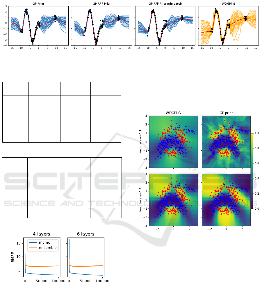
Figure 1: Sampled predictions of BNNs where the GP functional prior is imposed implicitly (our work) and by means of the

optimization of the Wasserstein distance with the functional BNN prior (WDGPi-G).

Table 1: Average RMSE for UCI regression datasets.

Dataset Functional WDGPi-G Deep

MCMC Ensembles

Boston 2.73±0.02 2.83±0.92 3.69±1.15

Concrete 4.06±0.12 4.80±0.41 5.22±0.63

Energy 0.48±0.18 0.34±0.07 1.37±0.32

Kin8nm 0.04±0.00 0.06±0.00 0.06±0.00

Power 3.24±0.06 3.72±0.18 3.86±0.21

Protein 3.61 ±0.04 3.65±0.02 4.45±0.02

Wine 0.60±0.01 0.60±0.04 0.62±0.02

Table 2: MNLL for UCI regression datasets.

Dataset Functional WDGPi-G Deep

MCMC Ensembles

Boston 2.45±0.01 2.48±0.12 3.19±1.12

Concrete 2.74±0.16 3.03±0.05 3.07±0.26

Energy 0.80±0.05 0.35±0.15 2.07±0.98

Kin8nm -1.46±0.11 -1.23±0.01 -1.32±0.08

Power 2.73±0.08 2.74±0.04 2.74±0.05

Protein 2.73±0.01 2.75±0.00 2.80±0.01

Wine 0.76±0.04 0.92±0.06 1.08±0.20

Ensembles over iterations (Fig. 2).

Figure 2: Convergence of RMSE on test data for the Power

dataset.

4.3 Toy Classiﬁcation Dataset

We demonstrate the proposed approach on a 2D toy

example using the banana dataset and a two-hidden

layer NN with tanh activation and 256 neurons per

layer. We transform the labels using the method from

(Milios et al., 2018) to allow for a Gaussian likeli-

hood, as described in Sec. 3. We use an RBF kernel

with σ

out

= 5 and varying length-scales, and compare

to the WDGPi-G method from (Tran et al., 2022). We

use a grid of 40×40 points as a regularization set and

test set. The plot shows that WDGPi-G fails to incor-

porate the GP prior for a small length-scale (l = 0.1)

and the prediction function is smoother than expected.

Figure 3: Sampled predictions of the neural network with

GP prior using Mahalanobis regularization and WDGPi-G

methods.

4.4 UCI Classiﬁcation Datasets

In this section, we test our approach on various UCI

classiﬁcation datasets using a two-hidden layer NN

with tanh activation. We use 100 neurons in each hid-

den layer for EEG, HTRU2, Letter, and Magic, and

200 neurons for Miniboo, Drive, and Mocap. We use

the RF approximation of the functional GP prior with

D = 1000 random features and mini-batches of size

512 on all datasets. GP hyper-parameters are opti-

mized using the label transformation from Sec. 3. We

found that using this transformation with the BNN it-

self gave slightly better results than using classiﬁca-

tion likelihoods, so we report these results in the ta-

ble. We attribute this to the optimization of GP hyper-

parameters with the transformed labels.

Imposing Functional Priors on Bayesian Neural Networks

455

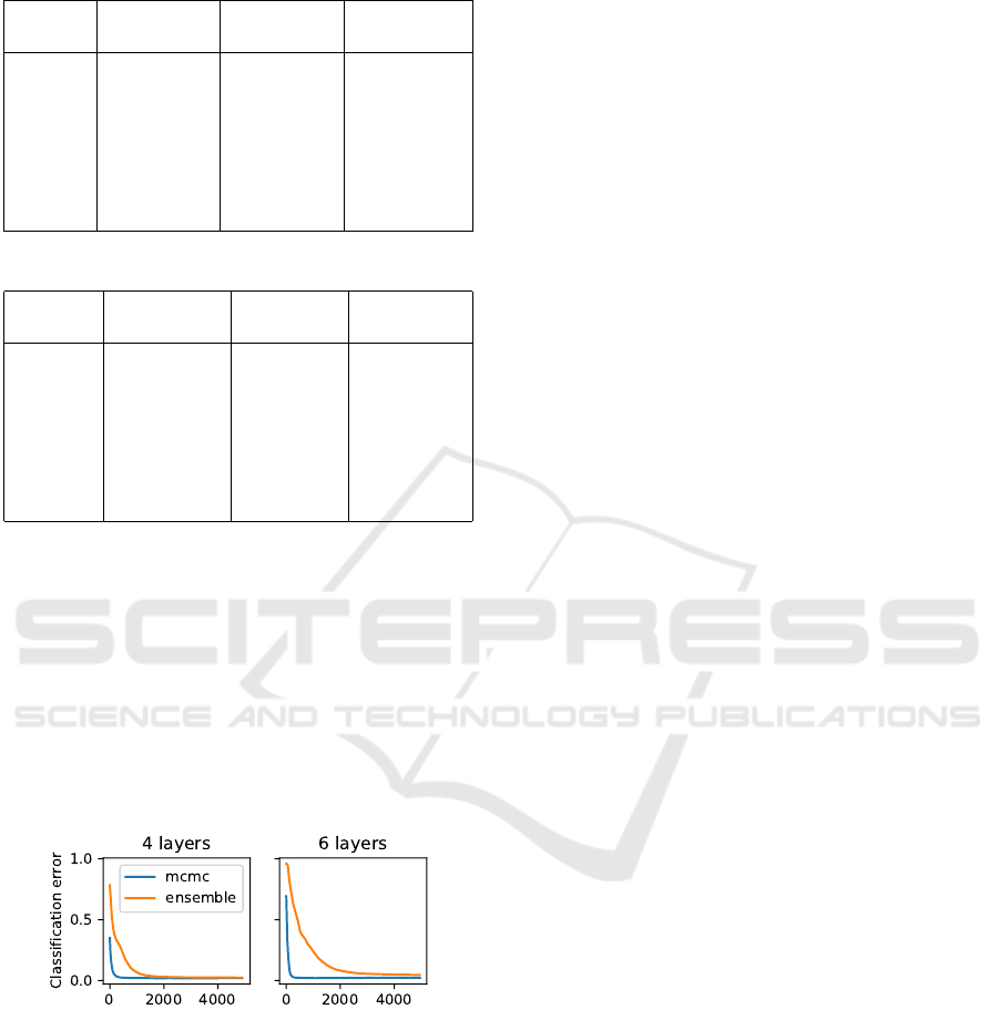
Table 3: Average classiﬁcation accuracy for UCI classiﬁca-

tion datasets.

Dataset Functional WDGPi-G Deep

MCMC Ensembles

EEG 92.51±1.82 94.13±1.96 89.04 ± 5.01

HTRU2 98.10±0.26 98.03±0.24 98.03 ± 0.20

Magic 88.16±0.33 88.37±0.29 87.90 ± 0.24

Miniboo 92.54±0.21 92.74±0.39 91.49 ± 0.19

Letter 98.22±0.18 96.90±0.29 96.38 ± 0.30

Drive 99.45±0.09 99.69±0.04 99.33 ± 0.05

Mocap 99.10±0.12 99.24±0.10 99.10 ± 0.08

Table 4: Average test NLL for UCI classiﬁcation datasets.

Dataset Functional WDGPi-G Deep

MCMC Ensembles

EEG 0.33±0.04 0.18±0.04 0.24 ± 0.10

HTRU2 0.06±0.002 0.06±0.00 0.07 ± 0.01

Magic 0.31±0.00 0.29±0.00 0.30 ± 0.01

Miniboo 0.18±0.01 0.18±0.00 0.20 ± 0.01

Letter 0.09±0.01 0.17±0.00 0.15 ± 0.01

Drive 0.08±0.01 0.03±0.00 0.05 ± 0.01

Mocap 0.19±0.00 0.03±0.00 0.04 ± 0.00

We compare our approach with other classiﬁca-

tion methods and found that it performs competitively

with the state-of-the-art, as shown in Tables 3 and 4.

Our approach does not require the Wasserstein opti-

mization phase used in WDGPi-G, while still achiev-

ing similar classiﬁcation performance after optimiz-

ing GP hyperparameters.

We also tested the proposed method on the Let-

ter dataset using NNs with four and six hidden layers

and compared its convergence to the Deep Ensemble

approach in terms of classiﬁcation accuracy (Fig. 4).

Figure 4: Convergence of classiﬁcation error on test data

for the Letter dataset.

5 LIMITATIONS

While we consider our approach quite elegant in en-

coding prior information in the form of functional pri-

ors, we believe that it is important to point out some

limitations compared to other works.

One limitation is that the posterior distribution we

are targeting is approximate due the way we treat the

change of variables from weights to functions.

Another limitation is that the functional prior

needs to have a closed form. Even though the class

of functional priors which have this property is large,

this might be too restrictive in applications where it

is possible to sample from such priors but no closed

form is available. Prior works which perform a pre-

liminary optimization of the prior over the weights

(e.g., (Tran et al., 2022)) can operate on samples from

functional priors without the need to express these in

closed form.

Finally, the choice of a GP prior requires set-

ting its hyper-parameters. In this work, we resort

to marginal likelihood optimization, but it is possible

that this choice induces overﬁtting. One way around

this would be to include hyper-parameters in the set

of variables to be sampled in SG-HMC to obtain sam-

ples from their posterior at the expenses of having to

deal with a more costly MCMC sampling. Having

said that, there are situations where functional priors

are easy to elicit and express without the need to carry

out hyper-parameter optimization.

6 CONCLUSIONS

In this paper, we proposed a novel way to incorpo-

rate prior knowledge in Bayesian NNs (BNNs) in the

form of functional priors. In our view, such functional

priors implicitly determine priors over BNN weights,

and the proposed formulation yields an approximate

posterior over the weights from which it is possible

to sample through MCMC or any other approximate

inference techniques. In this paper, we studied the

scenario where functional priors are expressed in the

form of Gaussian processes (GPs), but our formula-

tion can handle any functional prior which can be ex-

pressed in closed form. We then discussed how to

scale our approach to handle large data sets by operat-

ing on mini-batches, despite the complications stem-

ming from the use of GP priors.

We tested our proposal on regression and classiﬁ-

cation tasks and compared it with state-of-the-art ap-

proaches to carry out inference and prior optimization

for BNNs. Our results demonstrate that the proposed

approach is competitive in terms of performance and

quantiﬁcation of uncertainty, while being easy to im-

plement.

We are currently investigating ways to handle GP

priors with priors over hyper-parameters for increased

ﬂexibility, and alternative ways to specify functional

priors. Furthermore, we are investigating applica-

tions of BNNs for image classiﬁcation tasks for which

BNN architectures use convolutional layers.

ICPRAM 2023 - 12th International Conference on Pattern Recognition Applications and Methods

456

ACKNOWLEDGEMENTS

MF gratefully acknowledges support from the AXA

Research Fund and the Agence Nationale de la

Recherche (grant ANR-18-CE46-0002 and ANR-19-

P3IA-0002).

REFERENCES

Blundell, C., Cornebise, J., Kavukcuoglu, K., and Wierstra,

D. (2015). Weight uncertainty in neural network. In

International conference on machine learning, pages

1613–1622. PMLR.

Chen, T., Fox, E., and Guestrin, C. (2014). Stochastic Gra-

dient Hamiltonian Monte Carlo. In Xing, E. P. and

Jebara, T., editors, Proceedings of the 31st Interna-

tional Conference on Machine Learning, volume 32

of Proceedings of Machine Learning Research, pages

1683–1691, Bejing, China. PMLR.

Cutajar, K., Bonilla, E. V., Michiardi, P., and Filippone, M.

(2017). Random feature expansions for deep Gaus-

sian processes. In Precup, D. and Teh, Y. W., editors,

Proceedings of the 34th International Conference on

Machine Learning, volume 70 of Proceedings of Ma-

chine Learning Research, pages 884–893. PMLR.

Dua, D. and Graff, C. (2017). UCI machine learning repos-

itory.

Fortuin, V. (2022). Priors in bayesian deep learning: A re-

view. International Statistical Review.

Fortuin, V., Garriga-Alonso, A., Wenzel, F., Ratsch, G.,

Turner, R. E., van der Wilk, M., and Aitchison, L.

(2021). Bayesian neural network priors revisited.

In Third Symposium on Advances in Approximate

Bayesian Inference.

Graves, A. (2011). Practical variational inference for neural

networks. In Shawe-Taylor, J., Zemel, R., Bartlett, P.,

Pereira, F., and Weinberger, K., editors, Advances in

Neural Information Processing Systems, volume 24.

Curran Associates, Inc.

Kallenberg, O. and Kallenberg, O. (1997). Foundations of

modern probability, volume 2. Springer.

Kanagawa, M., Hennig, P., Sejdinovic, D., and Sriperum-

budur, B. K. (2018). Gaussian processes and kernel

methods: A review on connections and equivalences.

arXiv preprint arXiv:1807.02582.

Lakshminarayanan, B., Pritzel, A., and Blundell, C. (2017).

Simple and scalable predictive uncertainty estimation

using deep ensembles. In Guyon, I., Luxburg, U. V.,

Bengio, S., Wallach, H., Fergus, R., Vishwanathan,

S., and Garnett, R., editors, Advances in Neural Infor-

mation Processing Systems, volume 30. Curran Asso-

ciates, Inc.

Ma, C., Li, Y., and Hernandez-Lobato, J. M. (2019). Vari-

ational implicit processes. In Chaudhuri, K. and

Salakhutdinov, R., editors, Proceedings of the 36th

International Conference on Machine Learning, vol-

ume 97 of Proceedings of Machine Learning Re-

search, pages 4222–4233. PMLR.

Milios, D., Camoriano, R., Michiardi, P., Rosasco, L.,

and Filippone, M. (2018). Dirichlet-based gaussian

processes for large-scale calibrated classiﬁcation. In

Bengio, S., Wallach, H., Larochelle, H., Grauman,

K., Cesa-Bianchi, N., and Garnett, R., editors, Ad-

vances in Neural Information Processing Systems,

volume 31. Curran Associates, Inc.

Neal, R. (1996). Bayesian learning for neural networks.

Lecture Notes in Statistics.

Rahimi, A. and Recht, B. (2007). Random features for

large-scale kernel machines. In Platt, J., Koller, D.,

Singer, Y., and Roweis, S., editors, Advances in Neu-

ral Information Processing Systems, volume 20. Cur-

ran Associates, Inc.

Rudner, T. G. J., Chen, Z., and Gal, Y. (2021). Rethinking

function-space variational inference in bayesian neu-

ral networks. In Third Symposium on Advances in Ap-

proximate Bayesian Inference.

Shi, J., Sun, S., and Zhu, J. (2018). A spectral approach to

gradient estimation for implicit distributions. In Dy, J.

and Krause, A., editors, Proceedings of the 35th Inter-

national Conference on Machine Learning, volume 80

of Proceedings of Machine Learning Research, pages

4644–4653. PMLR.

Sun, S., Zhang, G., Shi, J., and Grosse, R. (2019). Func-

tional Variational Bayesian Neural Networks. In In-

ternational Conference on Learning Representations.

Tran, B.-H., Rossi, S., Milios, D., and Filippone, M. (2022).

All you need is a good functional prior for bayesian

deep learning. Journal of Machine Learning Re-

search, 23(74):1–56.

Wenk, P., Gotovos, A., Bauer, S., Gorbach, N. S., Krause,

A., and Buhmann, J. M. (2019). Fast gaussian process

based gradient matching for parameter identiﬁcation

in systems of nonlinear odes. In Chaudhuri, K. and

Sugiyama, M., editors, Proceedings of the Twenty-

Second International Conference on Artiﬁcial Intelli-

gence and Statistics, volume 89 of Proceedings of Ma-

chine Learning Research, pages 1351–1360. PMLR.

Wenzel, F., Roth, K., Veeling, B., Swiatkowski, J., Tran, L.,

Mandt, S., Snoek, J., Salimans, T., Jenatton, R., and

Nowozin, S. (2020). How good is the Bayes poste-

rior in deep neural networks really? In III, H. D. and

Singh, A., editors, Proceedings of the 37th Interna-

tional Conference on Machine Learning, volume 119

of Proceedings of Machine Learning Research, pages

10248–10259. PMLR.

Williams, C. K. and Rasmussen, C. E. (2006). Gaussian

processes for machine learning, volume 2. MIT press

Cambridge, MA.

Imposing Functional Priors on Bayesian Neural Networks

457