Evaluation of Factors-of-Interest in Bone Mimicking Models Based

on DFT Analysis of Ultrasonic Signals

Aleksandrs Sisojevs

, Alexey Tatarinov

and Anastasija Chaplinska

Institute of Electronics and Computer Science, 14 Dzerbenes Str., Riga, Latvia

Keywords: Pattern Recognition, DFT, Bone Models, Axial Quantitative Ultrasound.

Abstract: Bone fragility in osteoporosis is associated with a decrease in the thickness of the cortical layer CTh in long

bones and the development of internal porosity P in it. In the present work, an attempt was made to predict

the factors-of-interest CTh and P based on the pattern recognition approach, where DFT analysis was applied

to ultrasonic signals in surface transmission through a soft tissue layer. Compact bone was modeled with

PMMA plates with gradual changes in CTh from 2 to 6 mm, and internal porosity P was created by drilling

where the thickness of the porous layer P varied from 0 to 100% of CTh. The estimation method was based

on a statistical analysis of the magnitude of the DFT spectrum of the ultrasonic signals. Decision rules were

mathematical criteria calculated as ratios between the envelope functions of the magnitudes. Each of the

objects was chosen in turn as a test object, while other specimens composed the training set. The results of

the experiments showed the potential effectiveness of the CTh and P prediction, while additional physical

parameters may be used as decision rules to improve the reliability of the diagnosis.

1 INTRODUCTION

Osteoporosis is a systemic skeletal disease

characterized by low bone density and

microarchitectural deterioration of bone tissue with a

consequent increase in bone fragility (WHO, 2003).

It is a severe symptom of aging and a complication in

many metabolic diseases. Cortical bone or compact

bone tissue, the main load-carrying component of the

skeleton, suffers from osteoporosis by reducing the

thickness of the compact layer and increasing the

internal porosity in it, progressing from the side of the

channel (Osterhoff et al., 2016). An adequate

assessment of these manifestations of osteoporosis

can help in timely prevention and treatment.

Conventionally, the diagnosis of osteoporosis is made

using dual x-ray absorption techniques by measuring

the bone mineral density (Guglielmi, 2010).

However, planar radiography is not able to

distinguish reliably between changes associated with

bone thinning and porosity and thus distinguish

between thin normality and osteoporosis.

Ultrasonic techniques based on measuring the

parameters of elastic waves are a perspective

https://orcid.org//0000-0002-2267-4220

https://orcid.org//0000-0002-5787-2040

modality to assess bone conditions in respect of

osteoporosis (Laugier, 2008). Axial bone

ultrasonometers use to measure ultrasound velocity in

the compact bone of long bones, such as the tibia and

forearm bones. Although it demonstrated sensitivity

to osteoporosis and mineralization disorders, its

clinical use is compromised by the inability to discern

multiple factors influencing the bone condition by

this single input. New approaches are focused on

analysing guided wave propagation at several

frequencies that provide extensive information about

bone structure and properties (Tatarinov et al., 2014).

However, discrimination of the factors of interest

such as cortical porosity and thickness of the cortical

layer against the background of the influence of the

surrounding soft tissues requires advanced data

processing. Traditional approaches based on the

measurement of single parameters such as ultrasound

velocity do not allow separating the complex

influences of these acting factors. Artificial

intelligence methods, particularly, pattern recognition

applied to a complex of propagated ultrasonic signals

at different frequencies are expected to help solve the

problem.

914

Sisojevs, A., Tatarinov, A. and Chaplinska, A.

Evaluation of Factors-of-Interest in Bone Mimicking Models Based on DFT Analysis of Ultrasonic Signals.

DOI: 10.5220/0011742800003411

In Proceedings of the 12th International Conference on Pattern Recognition Applications and Methods (ICPRAM 2023), pages 914-919

ISBN: 978-989-758-626-2; ISSN: 2184-4313

 2023 by SCITEPRESS – Science and Technology Publications, Lda. Under CC license (CC BY-NC-ND 4.0)

The purpose of this study was to investigate the

possibility to detect differentially two independent

factors of interest, cortical thickness and intracortical

porosity as diagnostically valuable determinants of

bone fragility in osteoporosis. Synthetic solid

phantoms modeling the cortical layer with the gradual

variation of both factors were used. The very

formulation of the problem suggested the need to

apply pattern recognition methods, but unlike the

classical classification problem, in this case, there

was no need to determine the belonging of the object

under study to any known class, but just to find the

values of the factors, which were a-priori unknown.

Soft tissues covering bones were considered as an

aside factor, so the datasets were obtained for three

thicknesses of the soft layer to assure the feasibility

of the method for persons of different constitutions.

The raw data were presented by sets of ultrasonic

signals acquired stepwise by surface profiling of the

object in the pitch-catch mode. The discrete Fourier

transform (DFT), one of the recognized methods of

signal analysis, transforming the signals from time to

frequency domains was used (Irrigaray et al., 2016).

A set of statistical parameters was extracted from the

set of magnitude signals, thus forming a set of

features describing the object. Extracting statistical

parameters from each object in the set, decision rules

are created to be the instrument for the evaluation of

parameters of interest in the examined objects.

2 PROPOSED APPROACH

The proposed approach for evaluating two factors-of-

interest using ultrasonic signals datasets was based on

pattern recognition principles. The evaluation method

consisted of two parts: creating a set of decision rules

from the data for a training set of phantoms and

validating the set of decision rules by substitution the

data for an examination specimen to make verify the

correctness of the approach.

2.1 Bone Phantoms and Ultrasonic

Data Acquisition

Bone models (phantoms) presented a set of bi-layer

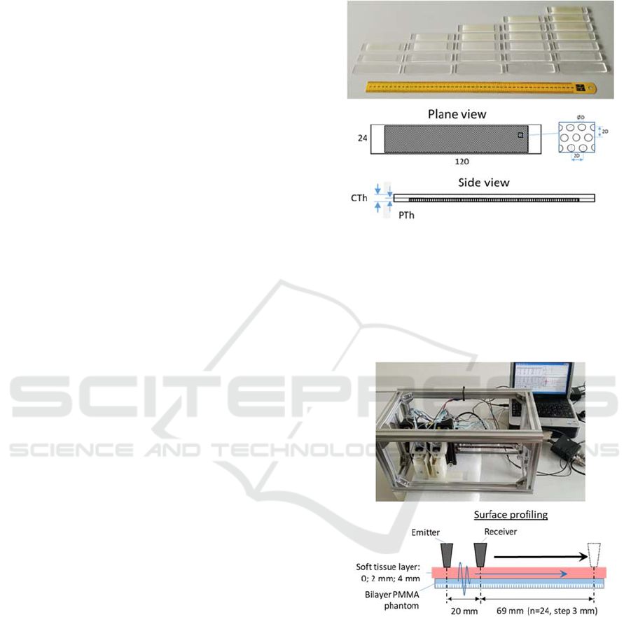
PMMA (polymethyl methacrylate) plates (Figure1)

with gradually varied overall thicknesses 2, 3, 4, 5

and 6 mm that corresponded to the bone cortical

thickness CTh. The effect of intracortical porosity

progressing from the in-bone channel was imitated by

the regularly bottom-drilled holes. The volumetric

porosity of the porous layer was constant at the level

of 20%, but the gradual progress of porosity P from

zero to 100% of CTh was set by increasing the

thickness of the porous layer PTh with a step of 1 mm.

Figure 1: PMMA phantoms modeling the progression of

osteoporosis in compact bone tissue: CTh – cortical

thickness; PTh – thickness of the porous layer.

Ultrasonic signals were acquired by means of a

custom-made scanning setup by stepwise profiling

the upper surface of the phantoms covered by soft

tissues with a profiling step of 3 mm (Figure 2).

Figure 2: Acquisition of ultrasonic signals in phantoms: A

– general view of ultrasonic setup, B – layout of

experiment.

Totally acquired 24 signals formed so called

ultrasonic spatiotemporal waveform profiles that

served as the source material for pattern recognition

(Figure 3). The profiles contained complex

information on temporal (velocities) and energetic

(attenuation) characteristics of different modes of

ultrasound propagation in the objects. Commonly, it

presents difficult to analyze those analytically using

signals decomposition (Bochud et al., 2017), but the

Evaluation of Factors-of-Interest in Bone Mimicking Models Based on DFT Analysis of Ultrasonic Signals

915

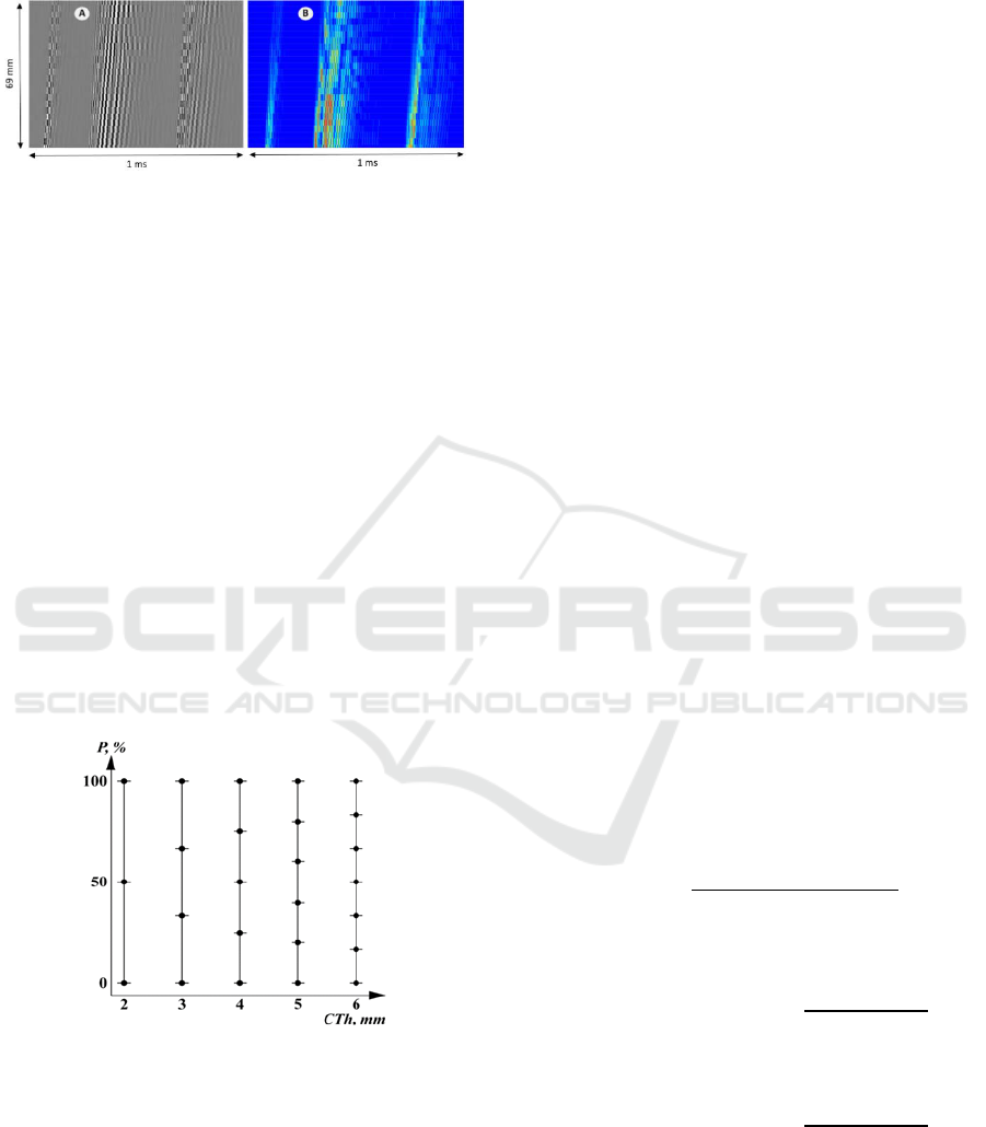
pattern recognition approach provided an integral

solution.

Figure 3: Examples of ultrasonic spatiotemporal waveform

profiles in bone phantoms: A – normalized within each

signal line; B – normalized upon the entire profile. The

abscissa is ultrasonic time; the ordinate is profiling

distance.

In one signal frame of a 1 ms duration, three

frequency excitation responses were collected: HF at

500 kHz, LF at 100 kHz, and a chirp signal with

frequency sweeping from 500 to 50 kHz. In this

frequency range, different modes of ultrasonic guided

waves manifested, including S0 and A0 Lamb waves.

2.2 Used Mathematical Method

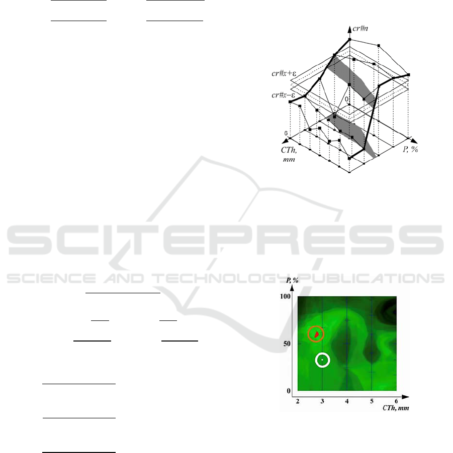
The initial data set comprised raw ultrasonic signals

obtained at three different frequency regimes of

excitation (HF, LF, chirp) and forming the

spatiotemporal waveform profiles that contained 24

stepwise acquired signals. The general structure of

the initial data on objects (phantoms) is shown in

Figure 4.

Figure 4: Data structure of source objects in the space of

factors-of-interest CTh and P.

As the set of bi-layer phantoms consisted of

gradually varied solid and porous layers with an

increment of 1 mm, the objects’ grid in the space of

the factors-of-interest CTh and P was a non-

orthogonal one that made an additional challenge for

interpolation.

In this study, the method for evaluating of factors

of interest used a pattern recognition approach

applied to ultrasonic signals after DFT processing

(Sisojevs et al., 2022). The signal frame consisting of

three frequency regimes was divided into three-time

sub-frames. In each sub-frame, mathematical criteria

were calculated. For this, the magnitude functions of

the DFT signals received from the corresponding sub-

frames were used. Then, for each object, mathematical

criteria were calculated that presented various ratios

between the envelope functions of signal magnitudes

(Sisojevs et al., 2022). The total number of

mathematical criteria for one sub-frame was 13, and

considering three sub-frames in the time domain, the

number of mathematical criteria for one object was 39.

After calculating the mathematical criteria for all

objects in the training set, decision rules were built.

In this case, mathematical criteria were used as

attributes for pattern recognition rules. For decision

rule creation, the bilinear interpolation of a patch of

the surface was used (Sisojevs et al., 2022).

3 EXPERIMENTS

As part of the validation of the proposed approach,

experiments were carried out to assess the total

thickness of the bone phantom CTh and the thickness

of the porous part P with a-priori known values of the

soft tissue thickness. In the experiment, the soft tissue

thicknesses were 0, 2 and 4 mm.

A separate experiment was carried out for each of

the soft tissue thickness values. The experiment

looked like this. Of all the scanned objects, one was

selected for the test sample. The rest made up the

training set. In this work, the method (Sisojevs et al.,

2022) was used. For each object, the magnitudes of

DFT signals were calculated for sub-frames in the

signal time domain.

𝑀



𝜔







𝑅𝑒



𝜔







𝐼𝑚



𝜔







where:

𝑅𝑒



𝜔



𝑠



𝑡



∙𝑐𝑜𝑠

2𝜋∙𝑡∙𝜔

𝑡



𝑡_𝑚𝑖𝑛



_

_

and

𝐼𝑚



𝜔



𝑠



𝑡



∙𝑠𝑖𝑛

2𝜋∙𝑡∙𝜔

𝑡



𝑡_𝑚𝑖𝑛



_

_

In the selected interval ω, the values of three functions

were calculated:

𝐹_𝑚𝑎𝑥



𝜔



𝑚𝑎𝑥



𝑀



𝜔





;

𝐹









𝑎𝑣𝑒𝑟𝑎𝑔𝑒



𝑀



𝜔





and

𝐹_𝑚𝑖𝑛



𝜔



𝑚𝑖𝑛



𝑀



𝜔





ICPRAM 2023 - 12th International Conference on Pattern Recognition Applications and Methods

916

Then, according to the values of these functions,

mathematical criteria were calculated:

First criteria cr#1 is the number of 𝜔 values that

fulfill the condition

𝐹









𝑎𝑣𝑒𝑟𝑎𝑔𝑒𝐹_𝑚𝑎𝑥



𝜔



,𝑐𝑟#1;

𝑐𝑟#2





_













_









; 𝑐𝑟#3



_





|





_









;

𝑐𝑟#4



_





|





_









; 𝑐𝑟#5



_





|





_









;

where:

𝑑𝐹_𝑚𝑎𝑥



𝜔



𝐹_𝑚𝑎𝑥



𝜔



𝐹_𝑚𝑎𝑥



𝜔1



𝑑𝐹_𝑎𝑣𝑟



𝜔



𝐹_𝑎𝑣𝑟



𝜔



𝐹_𝑎𝑣𝑟



𝜔1



𝑑𝐹_𝑚𝑖𝑛



𝜔



𝐹_𝑚𝑖𝑛



𝜔



𝐹_𝑚𝑖𝑛



𝜔1





𝑐𝑟#6

𝑐𝑟#7

𝑐𝑟#8





𝑊





∙

⎝

⎜

⎛

𝜔





∙𝐹_𝑚𝑎𝑥



𝜔





𝜔



∙𝐹_𝑚𝑎𝑥



𝜔





𝐹_𝑚𝑎𝑥



𝜔





⎠

⎟

⎞

where:



𝑊





⎝

⎜

⎛

𝜔







𝜔







𝜔







𝜔







𝜔







𝜔



𝜔







𝜔



𝜔



𝜔



⎠

⎟

⎞

𝑐𝑟#9

𝑚𝑎𝑥𝐹_𝑎𝑣𝑟



𝜔





𝑚𝑎𝑥𝐹_𝑚𝑎𝑥



𝜔





𝑐𝑟#10









; 𝑐𝑟#11









;

𝑐𝑟#12













; 𝑐𝑟#13













where:

𝑆





𝑚𝑎𝑥



𝐹_𝑚𝑎𝑥



𝜔





∙𝐹_𝑚𝑖𝑛



𝜔



_

_

𝑆





𝑚𝑎𝑥



𝐹_𝑚𝑎𝑥



𝜔





∙  𝐹_𝑎𝑣𝑟



𝜔



_

_

𝑆





𝑚𝑎𝑥



𝐹_𝑚𝑎𝑥



𝜔





∙𝐹_𝑚𝑎𝑥



𝜔



_

_

The interest parameter estimation method was

based on the creation and use of decision rules. To

create decision rules, piecewise linear interpolation

was used for each of the parametric directions. As a

result, the decision rule was represented as a

piecewise bilinear function of two variables.

The use of a decision rule to evaluate an unknown

object was reduced to the calculation of mathematical

criteria and their comparison with the corresponding

decision rules. In this case, the value of the criterion

expanded to the interval ±ε (eps). The result of

evaluation according to one rule is a set (segment) of

possible correct answers. Figure 5 illustrates such a

case.

Figure 5: An example of using a single decision rule to

evaluate an unknown object.

When using several decision rules, a sub-segment

of possible answers is found that is included in the

maximum number of initially found segments. It is

this sub-segment that is taken as the final evaluation

of the method used.

Figure 6: Result of evaluation of object with CTh = 3 mm

and P = 33.3% (PTh = 1 mm), soft tissue thickness = 0 mm

and eps = 25%.

After this estimate was obtained, this result was

compared with the a-priori known values of CTh and

P of this object. Within the framework of one

experiment, each of the objects was chosen in turn as

a test object.

Examples of how the method of the estimation

factors-of-interest works are shown in Figures 6-8. In

the figures, the red segment is the obtained estimate

Evaluation of Factors-of-Interest in Bone Mimicking Models Based on DFT Analysis of Ultrasonic Signals

917

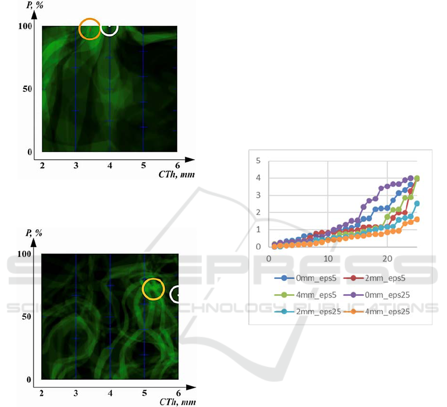
of the non-test object by the method (Sisojevs et al.,

2022), the white dot denotes the position of the test

object.

Figure 7: Result of evaluation of object with CTh = 4 mm,

P = 100% (PTh = 4 mm), soft tissue thickness = 2 mm and

eps = 25%.

Figure 8: Result of evaluation of object with CTh = 6 mm,

P = 66.6% (PTh = 4 mm), soft tissue thickness = 4 mm and

eps = 5%.

3.1 Estimation Accuracy

The estimation accuracy in the experiment was

determined for each of the factors-of-interest (CTh

and P). The error was calculated as the modulus of the

difference between the computed estimate of the

factor’s value and the a-priori known value of this

factor in the object

The estimate of the error in determining CTh

ranged from 0.0021 to 3.992 mm (i.e. between very

precise and completely incorrect). The average

estimation error was in the range of 0.561 - 1.675 mm

(depending on soft tissue thickness and eps value).

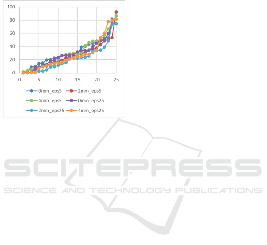
After sorting the errors in ascending order, the

distribution of errors is shown in Figure 9. The best

results or the results showing the smallest deviation

for CTh estimation are obtained with a value of the

soft tissue thickness layer of 4 mm and 2 mm at

eps=25% (average error 0.561 - 0.749 mm, maximum

1.606 - 2.532mm). Contrary, the worst results (the

highest deviation) are obtained for the value of the

soft tissue thickness layer 0 mm, regardless of the eps

value (average error 1.372 - 1.675 mm, maximum

3.623 - 3.983 mm). If the acceptable diagnostic

deviation threshold for CTh is 1.2 mm with a general

range of its changes from 2 to 6 mm, then the number

of correct estimations is 20 out of 25 or 80%.

Figure 9: Distribution of errors for CTh estimations

depending on the thickness of the soft tissue layer and eps.

The estimate of the error in determining the porosity

ranged from 0 to 92.478%, i.e. from the lowest to the

almost highest possible). The average estimation

error was in the range of 21.736 - 31.162%.

Depending on soft tissue thickness and eps value.

After sorting the errors in ascending order, the

distribution of errors for P is shown in Figure 10. The

best results from the point of least deviation for

porosity P were obtained with a soft tissue thickness

layer 2 mm at eps=25% (average error 21.736%,

maximum error 74.558%). At the same time, the

parameters (thickness of soft tissue and eps) giving

the worst performance in terms of accuracy are not

indicated. If the acceptable diagnostic deviation

threshold for P is 30% with a general range of its

changes from 0 to 100% mm, then the number of

correct estimations is 15 out of 25 or 60%. This shows

that the accuracy of determining bone thickness CTh

is somewhat better than that of its porosity P, using

CTh

ICPRAM 2023 - 12th International Conference on Pattern Recognition Applications and Methods

918

DFT-based criteria applied to the ultrasonic signals

related to the guided waves propagation.

Figure 10: Distribution of porosity P estimation errors

depending on the thickness of the soft tissue layer and eps.

4 CONCLUSIONS

The results of the experiments showed the potential

effectiveness of the earlier proposed pattern

recognition method (Sisojevs et al., 2022) in the tasks

of determining the factors of interest in osteoporosis

diagnostics (total thickness of the cortical bone and

the degree of inner porosity), using ultrasonic surface

profiling.

The use of only the DFT analysis does not give

full agreement between the obtained estimates and the

a priori predicted ones. The application of additional

evaluation criteria based on the physical parameters

of guided wave propagation may improve the

reliability of the diagnosis.

The small number of available objects (bone

phantoms) and the approximate nature of the

mathematical criteria did not allow us to estimate the

factors of interest with high accuracy. However, the

results obtained demonstrated the prospects for using

this method and increasing its accuracy with an

increase in the number of objects with a priori known

values of the factors.

ACKNOWLEDGEMENTS

The study was supported by the research project of

the Latvian Council of Science lzp-2021/1-0290

“Comprehensive assessment of the condition of bone

and muscle tissues using quantitative ultrasound”

(BoMUS).

REFERENCES

WHO Scientific Group on the Prevention and Management

of Osteoporosis (2000: Geneva, Switzerland). (2003)

Prevention and management of osteoporosis: report

of a WHO scientific group. WHO Technical Report

Series 921.

Osterhoff G, Morgan EF, Shefelbine SJ, Karim L,

McNamara LM, Augat P. (2016) Bone mechanical

properties and changes with osteoporosis. Injury.; 47,

Suppl 2: 11-20.

Guglielmi G, Scalzo G. (2010) Imaging tools transform

diagnosis of osteoporosis. Diagnostic Imaging Europe.

26: 7–11.

Laugier P. (2008) Instrumentation for in vivo ultrasonic

characterization of bone strength. IEEE Trans Ultrason

Ferroelectr Freq Control; 55(6):1179-96.

Tatarinov A, Egorov V, Sarvazyan N, Sarvazyan A. (2014)

Multi-frequency axial transmission bone

ultrasonometer. Ultrasonics. 54(5):1162-1169.

Irrigaray, M. A. P., Pinto R.C. and Padaratz I. J (2016) A

new approach to estimate compressive strength of

concrete by the UPV method. Revista IBRACON de

Estruturas e Materiais 9: 395-402.

Bochud N, Vallet Q, Minonzio JG, Laugier P. (2017)

Predicting bone strength with ultrasonic guided waves.

Sci Rep.; 7 (3):43628.

Sisojevs A., Tatarinov A., Kovalovs M., Krutikova O.,

Chaplinska A. (2022) An Approach for Parameters

Evaluation in Layered Structural Materials based on

DFT Analysis of Ultrasonic Signal. Proceedings of the

11th International Conference on Pattern Recognition

Applications and Methods, Volume 1: ICPRAM, 307-

314.

CTh

Evaluation of Factors-of-Interest in Bone Mimicking Models Based on DFT Analysis of Ultrasonic Signals

919