Joint Multi-Item Production and Condition-Based Maintenance
Control of a System with Setup Times and Stochastic Demand
Alp Darendeliler
1a
, Dieter Claeys
1,2 b
and El-Houssaine Aghezzaf
1,2 c
1
Department of Industrial Systems Engineering and Product Design, Ghent University, Ghent, Belgium
2
Industrial Systems Engineering (ISyE), Flanders Make, Kortrijk, Belgium
Keywords: Condition-Based Maintenance (CBM), Semi-Markov Decision Process (SMDP), Multi-Product,
Reinforcement Learning, Stochastic Demand.
Abstract: In this paper, we address the joint production and Condition-based maintenance (CBM) planning problem for
a deteriorating single-machine multi-product manufacturing system with uncertain product demands. The
objective is to find an integrated production and maintenance policy such that the sum of expected setup,
holding, lost sales, preventive and corrective maintenance costs is minimized. We formulate the problem as a
semi-Markov decision process and propose a Q-learning algorithm for the problem. A numerical example is
provided to illustrate the solution method.
1 INTRODUCTION
Preventive maintenance aims to reduce the likelihood
of equipment failures that result in unexpected
downtimes and production losses. Condition-based
maintenance (CBM), as a preventive maintenance
strategy, recommends performing maintenance
activities based on the current equipment condition.
If a CBM program is properly implemented, it can
significantly save costs by reducing the unnecessary
scheduled preventive maintenance operations
(Jardine et. al, 2006).
In recent years, the integration of production lot-
sizing and CBM has been studied by many
researchers. The majority of the existing research
studies the joint optimization of the economic
production quantity (EPQ) and CBM for single-
product systems under constant and deterministic
demand rate. However, there are many cases in
practice where multiple-items are produced by a
single facility (machine) and the demand is uncertain.
In this study, we consider a stochastically
degrading single-machine multi-product production/
inventory system under stochastic demand. Only a
single product can be produced at a time. The
produced items are stored in the inventory with
a
https://orcid.org/0000-0002-5217-7444
b
https://orcid.org/0000-0002-7666-2479
c
https://orcid.org/0000-0003-3849-2218
limited capacity for each product, and holding costs
are charged for the unconsumed products. Unsatisfied
demand is lost, and a penalty cost is incurred for each.
Switching production from one product to another or
from the idle state to production takes a certain
amount of time, and a setup cost is charged for this
operation. The degradation level of the machine
increases with production, and degradation behaviour
changes with respect to the product being produced.
Preventive or corrective maintenance brings the
machine to “as good as new” state and they both take
a deterministic time. The goal is to find a joint
production/inventory and maintenance policy to
minimize the long run expected average cost per unit
time, which includes the holding, lost sales, setup,
preventive and corrective maintenance costs.
We model the above-mentioned problem as a
semi-Markov decision process (SMDP), in which the
system state consists of the degradation level, the
setup status of the machine and the stock levels of the
products. Upon observing the state at a decision
epoch, one of the following actions is taken: keeping
the machine idle; producing a particular product that
the machine has been set up; carrying out setup for a
product in case the machine is idle or has been set up
for another product; performing preventive
Darendeliler, A., Claeys, D. and Aghezzaf, E.
Joint Multi-Item Production and Condition-Based Maintenance Control of a System with Setup Times and Stochastic Demand.
DOI: 10.5220/0011741300003396
In Proceedings of the 12th International Conference on Operations Research and Enterprise Systems (ICORES 2023), pages 185-192
ISBN: 978-989-758-627-9; ISSN: 2184-4372
Copyright
c
 2023 by SCITEPRESS – Science and Technology Publications, Lda. Under CC license (CC BY-NC-ND 4.0)
185

maintenance; or performing corrective maintenance
(it is the only choice if the machine fails). To solve
the underlying model, we adopt a Q-learning
algorithm for SMDP.
The rest of the paper is organized as follows. In
Section 2, we review the relevant literature. The
SMDP formulation is presented in Section 3. Then, in
Section 4, we present the Q-learning algorithm
adopted for our problem. In Section 5, a numerical
example is given. Then, concluding remarks are
provided in Section 6.
2 LITERATURE REVIEW
The integration of lot-sizing and time-based preventive
maintenance has been extensively studied by many
researchers (Aghezzaf et al., 2007; Ben Daya and
Makhdoum, 1998; Ben-Daya, 2002; El-Ferik, 2008;
Liao and Sheu, 2011; Suliman and Jawad, 2012;
Shamsaei and Vyve, 2017). In recent years, integrated
EPQ and CBM-based preventive maintenance models
have been proposed with the aim of optimizing the lot-
size and the degradation threshold, beyond which
preventive maintenance is conducted. Jafari and Makis
(2015) address the joint optimization of EPQ and
preventive maintenance policy. The deterioration of
the system is modelled by a proportional hazards
model that considers the condition monitoring
information and the age of the machine. Peng and van
Houtum (2016) develop a joint optimization model of
EPQ and CBM in which degradation is modelled as a
continuous time and continuous state stochastic
process. Khatab et al. (2019) investigate the problem
of integrating production quality and CBM for a
production system under periodic monitoring. Cheng
et al. (2018) develop a model to optimize production,
quality control and CBM policies for a system in which
product quality depends on the degradation level. Jafari
and Makis (2016) propose a model to jointly optimize
EPQ and preventive maintenance policy for a partially
observable two-unit system. Cheng et al. (2017)
consider joint optimization of production lot-sizing and
CBM for systems with multiple products. Preventive
maintenance decision making depends on the
predictive reliability and the structural importance
measure of the components.
Fewer studies, however, develop integrated
production and maintenance policies for systems with
stochastic demand. To find the optimal policy for
systems with stochastic demand, MDP and SMDP
models are proposed (Iravani and Duenyas, 2002;
Sloan, 2004; Jafari and Makis, 2019; Xiang et al.,
2014). These studies assume that the system produces
a single product type and the degradation is modelled
by a Markov chain with a limited number of states. In
this study, however, we propose a joint production
and CBM policy for a multi-product production
system with random product demands.
Darendeliler et al. (2022) has recently studied
joint optimal production/inventory and CBM control
for a multi-product manufacturing system under
stochastic product demands. It is assumed that the
system is reviewed at equidistant time points, so the
durations of producing a lot and maintenance are
assumed to be equal. The present paper relaxes this
assumption and extends the work by modelling the
problem as a SMDP, in which the system is reviewed
at the completion of a unit production, setup and
maintenance. Also, the previous work does not take
the production setup times into account, while they
are incorporated in the present model.
In literature, the problem of planning the lot-size
and sequence of several products on a single machine
with random product demands is known as the
stochastic economic lot scheduling problem
(SELSP). In the SELSP, the objective is to find a
policy that proposes whether to continue the
production of the current item, whether to switch to
another product or whether to keep the machine idle
so as to minimize the total expected average cost.
Obtaining such a policy, which dynamically
distributes the finite production capacity among the
products to be reactive to the stochastic demands,
processing and setup times, is a challenging problem
(Sox et al., 1999). Winands et al. (2011) categorize
SELSPs based on their sequencing and lot-sizing
strategies. Our model’s production policy could be
considered in the category of dynamic sequence and
global lot-sizing, in which there is no predetermined
production sequence, and the quantity of the lot-size
depends on the stock levels of all products and the
machine status rather than depending only on the
stock level of the product currently setup. The
majority of the SELSP models do not consider the
effect of equipment deterioration and maintenance on
the production policies. However, in this study, we
incorporate CBM policy in the SELSP problem.
There are few studies that consider dynamic
sequencing and global lot-sizing for the SELSP. Qiu
and Loulou (1995) model the SELSP as a SMDP and
solve limited-size problems by the successive
approximation method. Wang et al. (2012) apply two
reinforcement learning algorithms to the SELSP with
the random demand and processing times. Löhndorf
and Minner (2013) propose an approximate value
iteration method and compare its performance with the
global search for parameters of simple control policies.
ICORES 2023 - 12th International Conference on Operations Research and Enterprise Systems
186

3 PROBLEM FORMULATION
We consider a single machine production system
producing 𝑁 items one at a time. The processing time
of product 𝑛 takes 𝜌

time units, and the machine must
be set up for product 𝑛 if it is going to be produced.
The setup for item 𝑛 takes 𝑆𝑇

time units and incurs a
cost 𝑐𝑠

. Finished products are stored in an inventory
with limited storage capacity 𝑥̅

for each product 𝑛∈

1,…,𝑁

. A holding cost of 𝑐ℎ

is charged per
product per unit time for product 𝑛. Demand for each
product follows a Poisson process with rate 𝜆

. The
unsatisfied demand is lost and a lost sales cost 𝑐𝑙

is
incurred per item. The machine has multiple
degradation states

1,…,𝐹

, where 1 is the as-new
state, and 𝐹 is the failure state. If the machine
degradation level is observed to be 𝐹, then corrective
maintenance is immediately performed which takes
𝐶𝑇 time unit and costs 𝑐𝑐 . Conducting preventive
maintenance in an operational state takes 𝑃𝑇 time units
and costs 𝑐𝑝 . Both preventive and corrective
maintenance bring the machine to the as good as new
state (state “1”). Note that the system cannot be
interrupted during production, setup and maintenance
operations. The objective is to find the optimal
production/inventory and maintenance policy that
minimizes the total long-run average cost per time unit.
We formulate the problem as a semi-Markov
decision process (SMDP), where the state is
described as 𝑠=
(
𝑖,𝑘,𝑥

,…,𝑥

)
with degradation
level 𝑖∈

1,…,𝐹

, machine status 𝑘∈

0,…,𝑁

and
the product inventories 𝑥

,…,𝑥

. When the machine
status is 𝑘=𝑛, the machine has been set up for
product 𝑛∈

1,…,𝑁

. The system is reviewed at
decision epochs, which are epochs at which demand
for any product has just arrived in case the machine is
idle, or setup or production for an item has just been
completed, or preventive or corrective maintenance
has just been performed. At a decision epoch, based
on state 𝑠, an action 𝑎∈𝐴
(
𝑠
)
is chosen. The eligible
actions are: (1) keeping the machine idle
(
𝑎=0
)
; (2)
producing item 𝑛
(
𝑎=𝑛
)
; (3) carrying out
preventive maintenance
(
𝑎=−1
)
; (4) conducting
corrective maintenance ( 𝑎=−2) if and only if
failure occurs. If product 𝑛 is decided to be produced
and the machine is set up for another product or is in
the idle state, then the machine is going to be set up
for item 𝑛.
For state 𝑠=
(
𝑖,𝑘,𝑥

,…,𝑥

)
and action 𝑎, the
transition probabilities for the degradation can be
expressed as
𝑃

,
=
⎩
⎪
⎨
⎪
⎧
1𝑖𝑓𝑎=0,𝑖=
𝑗
1 𝑖𝑓 𝑎=−2 ,𝑖=𝐹,𝑗=1
1
𝑖𝑓 𝑎=−1,𝑗=1
𝑝

(
𝑛
) 𝑖𝑓 𝑎= 𝑛=𝑘,
𝑗∈

𝑖,…,𝐹

1𝑖𝑓𝑎=𝑛≠𝑘,
𝑗
=𝑖
0𝑜𝑡ℎ𝑒𝑟𝑤𝑖𝑠𝑒
,
(1
)
where, the degradation remains at the same level until
the next decision epoch if no production occurs, and
it will be at state 𝑗 in case of production.
The expected time until the next decision epoch is
given by
𝜏
(
𝑠,𝑎
)
=
⎩
⎪
⎪
⎨
⎪
⎪
⎧
1 𝜆

𝑓
𝑜𝑟 𝑎=0



𝐶𝑇 𝑓𝑜𝑟 𝑎=−2
𝑃𝑇 𝑓𝑜𝑟 𝑎=−1
𝜌

𝑓
𝑜𝑟 𝑎=𝑛 =𝑘
𝑆𝑇

𝑓
𝑜𝑟 𝑎=𝑛≠𝑘
.
(2
)
For state 𝑠=
(
𝑖,𝑘,𝑥

,…,𝑥

)
, the transition
probabilities of the stock level of product 𝑛=
1,…,𝑁, and the machine status 𝑘 under the action 𝑎
are as follows:
𝑇

(
𝑘

,𝑥


|
𝑘,𝑥

,𝑎
)
=
⎩
⎪
⎪
⎪
⎪
⎪
⎪
⎪
⎪
⎪
⎪
⎨
⎪
⎪
⎪
⎪
⎪
⎪
⎪
⎪
⎪
⎪
⎧
𝑃𝐷
𝑛
(
𝑡
)
=𝑥
𝑛
−𝑥
𝑛
′
 𝑓𝑜𝑟 𝑥
𝑛
′
>0,
𝑎=−2,−1;𝑘
′
=0∨
𝑎=𝑘≠𝑛>0,𝑘
′
=𝑎 ∨
𝑎≠𝑘>0,𝑘
′
=𝑎
𝑃
𝐷
𝑛
(
𝑡
)
≥𝑥
𝑛
−𝑥
𝑛
′
 𝑓𝑜𝑟 𝑥
𝑛
′
=0,
𝑎=−2,−1;𝑘
′
=0∨
𝑎=𝑘≠𝑛>0,𝑘
′
=𝑎 ∨
𝑎≠𝑘>0,𝑘
′
=𝑎
𝑃
𝐷
𝑛
(
𝑡
)
=𝑥
𝑛
−𝑥
𝑛
′
+1 𝑓𝑜𝑟 𝑥
𝑛
′
>1,
𝑎=𝑛=𝑘,𝑘
′
=𝑛
𝑃
(
𝐷
𝑛
(
𝑡
)
≥𝑥
𝑛
)
𝑓𝑜𝑟 𝑥
𝑛
′
=1
𝑎=𝑛=𝑘,𝑘
′
=𝑛
𝜆
𝑛
 𝜆
𝑗
𝑁
𝑗=1

𝑓𝑜𝑟 𝑥
𝑛
′
=
(
𝑥
𝑛
−1
)
+
𝑎=0,𝑘
′
=0
1−𝜆
𝑛
 𝜆
𝑗
𝑁
𝑗=1

𝑓𝑜𝑟 𝑥
𝑛
′
=𝑥
𝑛
,
𝑎=0,𝑘
′
=0
0 𝑜𝑡ℎ𝑒𝑟𝑤𝑖𝑠𝑒,
(3
)
Joint Multi-Item Production and Condition-Based Maintenance Control of a System with Setup Times and Stochastic Demand
187

where 𝑡=𝜏
(
𝑠,𝑎
)
and 𝐷

(
𝑡
)
is the random variable
with distribution 𝑃𝑜𝑖𝑠𝑠𝑜𝑛(𝜆

𝑡). For 𝑥


>0, if the
action is conducting corrective or preventive
maintenance
(
𝑎=−2,−1
)
, setup for any product
(
𝑎>0∧𝑎≠𝑘
)
or producing an item other than 𝑛
(
𝑎>0∧𝑎=𝑘≠𝑛
)
; then the transition probability
to the next state
(
𝑥


,𝑘

)
is 𝑃
(
𝐷

(
𝑡
)
=𝑥

−𝑥


)
; for
𝑥


=0, then the corresponding probability is
𝑃
(
𝐷

(
𝑡
)
≥𝑥

−𝑥


)
for the same actions. If
production takes place for product 𝑛 (𝑎=𝑛=𝑘),
then the transition probability to the next state is
𝑃
(
𝐷

(
𝑡
)
=𝑥

−𝑥


+1
)
when 𝑥


>1; for 𝑥


=1,
the transition probability is 𝑃
(
𝐷

(
𝑡
)
≥𝑥

−𝑥


+
1
)
. In case the machine is idle (𝑎=0), then the
inventory level at the next decision epoch is either
𝑥


=
(
𝑥

−1
)

with probability 𝜆

∑
𝜆



⁄
(first
demand is for item 𝑛) or 𝑥


=𝑥

with probability
1−𝜆

∑
𝜆



⁄
(the first arrival is demand for
another product).
Let 𝑆


,𝑆


,… denote demand arrival times for
product 𝑛. Then, the conditional expectation of 𝑆


,
given that 𝑚 demand arrivals occur in period of
length 𝑡, is given by
𝐸𝑆


𝐷

(
𝑡
)
=𝑚=
𝑡𝑗
𝑚+1
𝑓
𝑜𝑟 1≤
𝑗
≤𝑚.
(4)
By using the conditional expectation of arrival
times, the expected inventory holding cost for product
𝑛 , accumulated in a period of length 𝑡 , can be
expressed as
𝐻


𝑥

,𝑡

=𝑐ℎ


𝑡𝑗
𝑚+1
𝑃
(
𝐷

(
𝑡
)
=𝑚
)





+𝑐ℎ

𝑡
(
𝑥

−𝑚
)
𝑃
(
𝐷

(
𝑡
)
=𝑚
)





+𝑐ℎ


𝑡𝑗
𝑚+1
𝑃
(
𝐷

(
𝑡
)
=𝑚
)







.
(5)
The expected lost sales cost for product 𝑛 is given by
𝐿


𝑥

,𝑡

=𝑐𝑙


(
𝑚−𝑥

)
𝑃
(
𝐷

(
𝑡
)
=𝑚
)




.
(6)
𝐶(𝑠,𝑎) denotes the total expected cost incurred
until the next decision epoch if action 𝑎 is taken in
state 𝑠. It can be expressed as
𝐶
(
𝑠,𝑎
)
=
⎩
⎪
⎪
⎪
⎪
⎪
⎪
⎪
⎪
⎨
⎪
⎪
⎪
⎪
⎪
⎪
⎪
⎪
⎧
∑
𝑥

𝑐ℎ



∑
𝜆



+
∑
𝑐𝑙

(
1−𝑥

)



𝜆

∑
𝜆



𝑓𝑜𝑟 𝑎=0
𝑐𝑐+  𝐻


𝑥

,𝐶𝑇

+


𝐿


𝑥

,𝐶𝑇



𝑓𝑜𝑟 𝑎=−2
𝑐𝑝 +𝐻


𝑥

,𝑃𝑇

+


𝐿


𝑥

,𝑃𝑇



𝑓𝑜𝑟 𝑎=−1
𝐻


𝑥

,𝜌




+ 𝐿


𝑥

,𝜌




𝑓𝑜𝑟 𝑎=𝑚,𝑚=𝑘
𝑐𝑠

+𝐻


𝑥

,𝑆𝑇


+


𝐿


𝑥

,𝑆𝑇




𝑓
𝑜𝑟𝑎=𝑚,𝑚≠𝑘
.
(7)
The average cost optimality equation is as follows
𝑉
∗
(
𝑠
)
=min
∈
(

)

𝐶
(
𝑠,𝑎
)
−𝑔
∗
𝜏
(
𝑠,𝑎
)
+𝑃
(
𝑠

|
𝑠,𝑎
)


∈
𝑉
∗
(
𝑠

)
 ∀𝑠∈𝑆,
(8
)
where 𝑠=
(
𝑖,𝑘,𝑥

,…,𝑥

)
and 𝑠

=
(
𝑖

,𝑘

,𝑥


,…,𝑥


)
and the transition probability is
𝑃
(
𝑠

|
𝑠,𝑎
)
=𝑃


,
𝑇

(
𝑘

,𝑥


|
𝑘,𝑥

,𝑎
)
.


(9
)
A solution to these equations gives the minimum
expected average cost per time unit 𝑔
∗
and optimal
value functions 𝑉
∗
(
𝑠
)
. Any policy that minimizes the
right-hand side of (8) for all 𝑠∈𝑆 is optimal.
4 SOLUTION METHOD
Dynamic programming methods provide exact
optimal policies by iteratively solving the Bellman
equations. However, they are not computationally
feasible for large and even for moderate-size
problems. Hence, we apply the Q-learning algorithm
to our problem, which is a model-free reinforcement
learning algorithm proposed by Watkins (1989). Q-
learning estimates the optimal state-action values (Q-
values) by the sampled values instead of using
complete transition probabilities to make expected
updates.
ICORES 2023 - 12th International Conference on Operations Research and Enterprise Systems
188

1. Initialize a starting state 𝑠, and 𝑄(𝑠,𝑎) for all 𝑠∈𝑆 and action 𝑎∈ 𝐴(𝑠)
2. For 𝑡=1, 2,…,𝑇
2.1. Choose action 𝑎∈𝐴(𝑠) for state 𝑠 (𝜖− 𝑔𝑟𝑒𝑒𝑑𝑦)
2.2. Sample the cost 𝑐
(
𝑠,𝑎
)
, the sojourn time 𝜏 and the next state 𝑠

based on the current state 𝑠 and action 𝑎
2.3. Update the Q-value by the equation:
𝑄
(
𝑠,𝑎
)
←𝑄
(
𝑠,𝑎
)
+𝛼𝑐
(
𝑠,𝑎
)
+𝑒

min


∈(

)
𝑄
(
𝑠

,𝑎

)
−𝑄
(
𝑠,𝑎
)

2.4. Update 𝑠← 𝑠

3. Return 𝜇
(
𝑠
)
=𝑎𝑟𝑔𝑚𝑖𝑛
∈()
𝑄
(
𝑠,𝑎
)
𝑓
𝑜𝑟 𝑎𝑙𝑙 𝑠∈𝑆
Figure 1: Steps of Q-learning for SMDP.
We use the Q-learning algorithm adapted for
the SMDP (Bradtke and Suff, 1994), which is
proven to converge to an optimal policy if certain
conditions are satisfied (Parr, 1998). Figure 1 shows
the steps of the algorithm. First, the Q-values are
initialized to 0. Then, in Step 2, to balance
exploration and exploitation, an action is chosen for
current state 𝑠 according to the 𝜖− 𝑔𝑟𝑒𝑒𝑑𝑦 policy
in which the greedy action is taken with probability
(1 − 𝜖) and a random action is taken with
probability 𝜖. In Step 2.2, the realization of the
degradation path on the current state-action pair
and the product demands are sampled. By using
these values, the one period cost 𝑐
(
𝑠,𝑎
)
and the next
state 𝑠

are determined by the system equations
given in Appendix. Once these values are obtained,
the state-action value of the visited state-action pair,
𝑄
(
𝑠,𝑎
)
, is updated with the temporal difference
𝑐
(
𝑠,𝑎
)
+𝑒

min


∈(

)
𝑄
(
𝑠

,𝑎

)
−𝑄
(
𝑠,𝑎
)
 , where
𝜏 is the sampled sojourn time to the next iteration, and
𝛾 is the discount factor which is chosen to be
sufficiently small in order to minimize the average
cost. Note that the learning rate, 𝛼 , satisfies the
necessary conditions for optimality (Parr, 1998).
5 NUMERICAL EXAMPLE
In this section, we consider a manufacturing system
that produces three products
(
𝑁=3
)
. For each
product 𝑛, the storage capacity is 𝑥̅

=20. The setup
costs are set to zero as they mainly correspond to the
time lost when the system in not operating, which is
represented by the setup times. For each product, the
randomly generated parameters within the specific
ranges are shown in Table 1. The machine
degradation follows a gamma Process with shape 𝛼=
0.5 and scale parameter 𝛽=1, and the failure
threshold is 𝐿=10. Based on the procedure
proposed by De Jonge (2019), the gamma process is
approximated by a discrete-time Markov Chain with
21 states where 1 is the as-new state and 21 is the
failure state 𝐹.
Table 1: Problem parameters.
Paramete
r
Value
Demand rates
U
(
0.1,0.25
)
Production rates
U
(
1,2
)
Preventive maintenance time U
(
4,8
)
Corrective maintenance time U
(
10,16
)
Setup time U
(
0.5,2
)
Preventive maintenance cost
U
(
300,500
)
Corrective maintenance cost
U
(
800,1000
)
Holdin
g
costs
U
(
0.5,2
)
Lost sales costs U
(
100,200)
In the Q-learning algorithm, the actions are selected
according to 𝜖 − 𝑔𝑟𝑒𝑒𝑑𝑦 policy. Initially, we set 𝜖 to
0.1, then every 10

iterations, it is reduced by 𝜖←
0.9 × 𝜖. In updating the Q-values, the harmonic
learning rate, 𝛼=𝑏
(
𝑏+𝑁

(
𝑠,𝑎
)
−1
)⁄
with 𝑏=5,
is used, where 𝑁

(
𝑠,𝑎
)
is the number of times that a
state action pair
(
𝑠,𝑎
)
has been visited up to the time
𝑡; the parameter 𝑏 is tuned based on the procedure in
Powell (2011). Figure 2 shows the learning curve for
the Q-learning. The convergence of the average cost
rate towards the end of the simulation indicates that
the algorithm has reached a stable policy. The
solution algorithm is implemented in Wolfram
Mathematica 12. The computational experiment took
223.35 minutes on a quad-core Intel i7 processor
running at 1.80 GHz with 16 GB RAM.
6 CONCLUSIONS
In this paper, we have addressed the joint
optimization of production, inventory and CBM for a
stochastically degrading multi-product production
system with considerable setup and maintenance
times under stochastic product demands. The goal is
to find a dynamic production and maintenance policy
so as to minimize the long run average cost per time
Joint Multi-Item Production and Condition-Based Maintenance Control of a System with Setup Times and Stochastic Demand
189

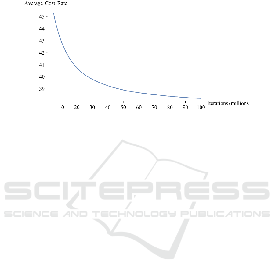
Figure 2: Learning curve of the Q-learning.
unit, which contains setup, holding, lost sales,
preventive maintenance and corrective maintenance
costs. The problem has been formulated as a SMDP,
in which decisions are made based on the current
machine status and stock levels of the products. To
solve this problem, we have proposed a Q-learning
algorithm and illustrate its performance by a
numerical example.
REFERENCES
Aghezzaf E-H., Jamali M., and Ait-Kadi D. (2007). An
integrated production and preventive maintenance
planning model. European Journal of Operational
Research, 181 (2), 679–685.
Ben-Daya M., and Makhdoum M. (1998). Integrated
production and quality model under various preventive
maintenance policies. Journal of the Operational
Research Society, 49(8), 840-853.
Ben-Daya M. (2002). The economic production lot-sizing
problem with imperfect production processes and
imperfect maintenance. International Journal of
Production Economics, 76 (3), 257–264.
Bradtke J.A, and Moore, A.W. (1995). Reinforcement
learning methods for continuous-time Markov decision
problems. In Advances in Neural Information Processing
Systems 7: Proceedings of the 1994 Conference
Denver, Colorado. MIT Press.
Cheng G.Q., Zhou B.H., and Li L. (2017). Joint
optimization of lot sizing and condition-based
maintenance for multi-component production systems.
Computers & Industrial Engineering, 110, 538-549.
Cheng G.Q., Zhou B.H., and Li L. (2018). Integrated
production, quality control and condition-based
maintenance for imperfect production systems.
Reliability Engineering & System Safety, 175, 251–264.
Darendeliler A., Claeys D., and E.H. Aghezzaf (2022).
Integrated condition-based maintenance and multi-item
lot-sizing with stochastic demand. Journal of Industrial
and Management Optimization. (In press).
De Jonge B. (2019). Discretizing continuous-time
continuous-state deterioration processes, with an
application to condition-based maintenance. Reliability
Engineering & System Safety, 188, 1-5.
El-Ferik S. (2008). Economic production lot-sizing for an
unreliable machine under imperfect age-based
maintenance policy. European Journal of Operational
Research, 186(1), 150–163.
Iravani S., and Duenyas I. (2002). Integrated maintenance
and production control of a deteriorating production
system. IIE Transactions, 34(5), 423–435.
Jafari L., and Makis V. (2015). Joint optimal lot sizing and
preventive maintenance policy for a production facility
subject to condition monitoring. International Journal
of Production Economics, 169, 156-168.
Jafari L., and Makis V. (2016). Joint optimal lot sizing and
maintenance policy for a partially observable two-unit
system. The International Journal of Advanced
Manufacturing Technology, 87, 1621-1639.
Jafari L., and Makis V. (2019). Optimal production and
maintenance policy for a partially observable
production system with stochastic demand.
International Journal of Industrial and Systems
Engineering, Vol:13, No:7.
Jardine A., Lin D., and Banjevic D. (2006). A review on
machinery diagnostics and prognostics implementing
condition-based maintenance. Mechanical Systems and
Signal Processing, 20, 1483–1510.
Khatab A., Diallo C., Aghezzaf E-H., and Venkatadri U.
(2019). Integrated production quality and condition-
based maintenance for a stochastically deteriorating
manufacturing system. International Journal
Production Research, 57(8), 2480-2497.
Liao G.L., and Sheu S.H. (2011). Economic production
quantity model for randomly failing production process
with minimal repair and imperfect maintenance.
ICORES 2023 - 12th International Conference on Operations Research and Enterprise Systems
190

International Journal of Production Economics, 130,
118-124.
Löhndorf N., and Minner S. (2013). Simulation
optimization for the stochastic economic lot scheduling
problem. IIE Transactions, 45, 796-810.
Parr R.E. (1998). Hierarchical control and learning for
Markov decision processes. PhD diss., University of
California at Berkeley.
Peng H., and van Houtum G.-J. (2016). Joint Optimization
of Condition-based Maintenance and Production Lot-
sizing. European Journal of Operational Research,
253, 94–107.
Powell W.B. (2011). Approximate Dynamic Programming.
Second edition. John Wiley & Sons.
Qiu J., and Loulou R. (1995). Multiproduct
production/inventory control under random demands.
IEEE Transactions on Automatic Control, 40(2), 350–
356.
Shamsaei F., and Van Vyve M. (2017). Solving integrated
production and condition-based maintenance planning
problems by MIP modeling. Flexible Services and
Manufacturing Journal, 29, 184-202.
Sloan T.W. (2004). A Periodic Review Production and
Maintenance Model with Random Demand,
Deteriorating Equipment, and Binomial Yield. Journal
of the Operational Research Society, 55(6), 647–656.
Sox C.R., Jackson P.L., Bowman A., and Muckstadt J.A.
(1999). A review of the stochastic lot scheduling
problem. International Journal of Production
Economics, 62(3), 181-200.
Suliman S.M., and Jawad S.H. (2012). Optimization of
preventive maintenance schedule and production lot
size. International Journal of Production Economics,
137, 19-28.
Wang. J., Xueping L., and Xiotan Z. (2012). Intelligent
dynamic control of stochastic economic lot scheduling
by agent-based reinforcement learning. International
Journal of Production Research, 50(16), 4381-4395.
Watkins C.J. (1989). Learning from delayed rewards. PhD
diss, Cambridge: Kings College.
Winands E., Adan I., and van Houtum G.J. (2011). The
stochastic economic lot scheduling problem: A survey.
European Journal of Operational Research, 201(1), 1–
9.
Xiang Y., Cassady C.R., Jin T., and Zhang C.W. (2014).
Joint production and maintenance planning with
machine deterioration and random yield. International
Journal Production Research, 52(6),1644–1657.
APPENDIX
The system evolves as follows: At a decision epoch,
upon observing the state 𝑠=
(
𝑖,𝑘,𝑥

,…,𝑥

)
, one of
the following actions can be chosen: (1) perform
corrective maintenance if and only if failure occurs;
(2) perform preventive maintenance; (3) keep the
machine idle; (4) produce item 𝑚. Then, based on
state 𝑠=
(
𝑖,𝑘,𝑥

,…,𝑥

)
, the selected action 𝑎∈
𝐴
(
𝑠
)
, the sampled degradation path and the demand
values (also the arrival times), the one-period cost
𝑐
(
𝑠,𝑎
)
and the next state 𝑠

=
(
𝑖

,𝑘

,𝑥


,…,𝑥


)
are
determined by the following equations:
Let,
𝜏: time until the next decision epoch,
𝑑

: sampled demand for product 𝑛 from
𝑃𝑜𝑖𝑠𝑠𝑜𝑛
(
𝜆

𝜏
)
for 𝑛=1,…,𝑁,
𝑆


: sampled 𝑟

demand arrival time for
𝑟=1,…,𝑑

and for product 𝑛=1,…,𝑁,
𝑤

=𝑚𝑖𝑛

𝑥

,𝑑


for product 𝑛=1,…,𝑁,
1. If 𝑖=𝐹 and corrective maintenance is being
performed (𝑎=−2), then
𝜏=𝐶𝑇,
𝑐
(
𝑠,𝑎
)
=𝑐

+
1 − 𝑒




𝛾
𝑐ℎ






+
(
1−𝑒

)
𝛾
𝑐ℎ

(
𝑥

−𝑤

)


+  𝑒



𝑐𝑙







,
𝑖

=1,𝑘

=0,𝑥


=
(
𝑥

−𝑑

)

,
…,𝑥


=
(
𝑥

−𝑑

)

.
2. If 𝑖<𝐹 and preventive maintenance is being
performed (𝑎=−1), then
𝜏=𝑃𝑇,
𝑐
(
𝑠,𝑎
)
=𝑐

+
1 − 𝑒




𝛾
𝑐ℎ






+
(
1−𝑒

)
𝛾
𝑐ℎ

(
𝑥

−𝑤

)


+  𝑒



𝑐𝑙







,
𝑖

=1,𝑘

=0,𝑥


=
(
𝑥

−𝑑

)

,
…,𝑥


=
(
𝑥

−𝑑

)

.
3. If 𝑖<𝐹 and the machine is being kept idle (𝑎=
0), then, let 𝑆
∗
=𝑚𝑖𝑛

𝑆


,…,𝑆



, and 𝑆


=𝑆
∗
, for
some 𝑟∈

1,…,𝑁

, then
𝜏=𝑆
∗
,
𝑐
(
𝑠,𝑎
)
=
(
1−𝑒

)
𝛾
𝑐ℎ

𝑥



+𝑒

𝑐𝑙

(
1−𝑥

)

,
𝑖

=𝑖,𝑘

=0,𝑥


=
(
𝑥

−1
)

.
𝑥


=𝑥

𝑓𝑜𝑟 𝑚∈

1,…,𝑁

∖𝑟
Joint Multi-Item Production and Condition-Based Maintenance Control of a System with Setup Times and Stochastic Demand
191

4. If 𝑖<𝐹 and product 𝑚 is going to be produced
(𝑎=𝑚), then
4.1. If 𝑎=𝑚=𝑘,
𝜏=𝜌

,
𝑐
(
𝑠,𝑎
)
=
1 − 𝑒




𝛾
𝑐ℎ






+
(
1−𝑒

)
𝛾
𝑐ℎ

(
𝑥

−𝑤

)


+  𝑒



𝑐𝑙








,
𝑖

≥𝑖, 𝑘

=𝑚,𝑥


=
(
𝑥

−𝑑

)

,
…,
(
𝑥

−𝑑

)

+1,…,𝑥


=
(
𝑥

−𝑑

)

.
4.2. If 𝑎=𝑚≠𝑘,
𝜏=𝑆𝑇

,
𝑐
(
𝑠,𝑎
)
=𝑐𝑠

+
1 − 𝑒




𝛾
𝑐ℎ






+
(
1−𝑒

)
𝛾
𝑐ℎ

(
𝑥

−𝑤

)


+  𝑒



𝑐𝑙







,
𝑖

=𝑖,𝑘

=𝑚,𝑥


=
(
𝑥

−𝑑

)

,
…,
(
𝑥

−𝑑

)

,…,𝑥


=
(
𝑥

−𝑑

)

.
ICORES 2023 - 12th International Conference on Operations Research and Enterprise Systems
192