Data Streams: Investigating Data Structures for Multivariate

Asynchronous Time Series Prediction Problems

Christopher Vox

, David Broneske

, Istiaque Mannafee Shaikat

and Gunter Saake

Volkswagen AG, Wolfsburg, Germany

German Centre for Higher Education Research and Science Studies, Hannover, Germany

Otto-von-Guericke-Universit

at Magdeburg, Magdeburg, Germany

Keywords:

Multivariate Asynchronous Time Series, Deep Learning, Convolutional Neural Network, Recurrent Neural

Network.

Abstract:

Time series data are used in many practical applications, such as in the area of weather forecasting or in the

automotive industry to predict the aging of a vehicle component. For these practical applications, multivariate

time series are present, which are synchronous or asynchronous. Asynchronicity can be caused by different

record frequencies of sensors and often causes challenges to the efﬁcient processing of data in data analytics

tasks. In the area of deep learning, several methods are used to preprocess the data for the respective models

appropriately. Sometimes these data preprocessing methods result in a change of data distribution and thus, to

an introduction of data based bias.

Therefore, we review different data structures for deep learning with multivariate, asynchronous time series

and we introduce a lightweight data structure which utilizes the idea of stacking asynchronous data for deep

learning problems. As data structure we create the Triplet-Stream with decreased memory footprint, which

we evaluate for one classiﬁcation problem and one regression problem. The Triplet-Stream enables excellent

performance on all datasets compared to current approaches.

1 INTRODUCTION

Time series data are generated, gathered and pro-

cessed all over the world. Thereby, these data are

of diverse nature, as there are, among others, peri-

odically sent short text messages, employees avail-

ability recordings, measurements of patient data for

clinical purposes, but also manifold sensor measure-

ments, which enable digitalized and autonomous ser-

vices. If we consider one recording at a speciﬁc time

point, then this measurement can have different di-

mensionality, such as images or text messages result

in value matrices and value vectors, whereas temper-

ature sensors generate one value per time point. The

time series evaluated within this work can be repre-

sented by the measurement information I : {(x,t) ⊆

I| x

(n,m)

∈ R

, t ∈ R

}. The measurement x is deﬁned

by the three-dimensional space spanned over n,m, z.

In the following, we limit ourselves to measurements

of one dimensional nature (n = m = z = 1) at a certain

time point t.

A speciﬁc challenge is that the introduced infor-

mation I can have different properties such as missing

or incorrect measurements (Sun et al., 2020; Weer-

39.8

40.1

40.2

40.1

𝑡

100

101.5

104

105 106

𝑡

1 0

𝑡

Vehicle Temperature Sensor (𝑆

)

Vehicle Speed Sensor (𝑆

)

Vehicle Light Sensor (𝑆

)

°C

time

km/h

time

On/Off

time

Figure 1: Characteristic of vehicle sensor data.

akody et al., 2021). Furthermore, measurements

from different sources can have different record fre-

quencies, which causes an asynchronous multivariate

space (Vox et al., 2022). According to (Wu et al.,

2018), multivariate time series data can be character-

ized as synchronous or asynchronous, as regular or

irregular and as co-cardinal or multi-cardinal. Asyn-

chronicity can be deﬁned as multivariate time series

state, where the measurements of the univariate time

series are not synchronized to a uniform time pat-

tern and thus not aligned on the time domain. More-

over, when the amount of measurements of univariate

time series within a multivariate time series space are

different, the time series space can be described as

686

Vox, C., Broneske, D., Shaikat, I. and Saake, G.

Data Streams: Investigating Data Structures for Multivariate Asynchronous Time Series Prediction Problems.

DOI: 10.5220/0011737300003411

In Proceedings of the 12th International Conference on Pattern Recognition Applications and Methods (ICPRAM 2023), pages 686-696

ISBN: 978-989-758-626-2; ISSN: 2184-4313

 2023 by SCITEPRESS – Science and Technology Publications, Lda. Under CC license (CC BY-NC-ND 4.0)

multi-cardinal. In addition, when all univariate time

series have the same amount of measurement points,

the multivariate time series space is co-cardinal.

The data source we investigate is shown in Fig-

ure 1. Three different sensors (one temperature sensor

), one speed sensor (S

) and one light control sen-

sor (S

)) are presented, which have unevenly spaced

measurements due to an event-based recording. Thus,

the multivariate sensor space is asynchronous, multi-

cardinal and irregular but is referred to in simpliﬁed

terms as asynchronous time series in the following.

As already introduced, different variations of time

series exist whereby the investigation of this work is

based on time series of one-dimensional characteris-

tic. The investigation covers two prediction problems

in the context of Multivariate asynchronous Time Se-

ries (MaTS). The ﬁrst prediction problem is based

on a clinical dataset, which describes the in-hospital

mortality of patients. The second problem under in-

vestigation is based on a vehicle component aging

dataset.

Within literature, different models have been in-

troduced, which solve the prediction problems with

complex model architectures or with the help of syn-

chronizing aggregations (Che et al., 2018; Sass et al.,

2019; Horn et al., 2020; Shukla and Marlin, 2021).

Particularly, over the last years the depth of Deep

Neural Networks (DNNs) grew signiﬁcantly to opti-

mize the reliability and the goodness of estimation. In

contrast, (Schwartz et al., 2020) elaborated the impor-

tance of the consideration of the efﬁciency of machine

learning to minimize the required computational ef-

fort. They identiﬁed that only a small percentage of

publications evaluated by them focused on the efﬁ-

ciency of deep Artiﬁcial Neural Networks (ANNs)

also called DNNs. Especially, with respect to sustain-

ability and with regard to the rebound effects of dig-

italization, machine learning models should process

time series data efﬁciently. Hence, the focus of the

development of DNNs should be on small and opti-

mized models with reduced data preprocessing effort.

One beneﬁt of this optimization can be an efﬁcient

and highly optimized continuous operation of DNNs.

For this purpose, we investigate present data struc-

tures for DNNs which are used to solve prediction

problems based on MaTS. Likewise, we evaluate the

models that utilize the data structures, based on their

performance and capacity. On the basis of the estab-

lished solutions, we develop a lightweight but highly

efﬁcient data structure to solve asynchronous time se-

ries prediction problems. The main contributions of

this paper are as follows:

• Investigating data structures and models for pre-

diction problems based on MaTS. Focusing on

introduced bias by manipulating the data distribu-

tion and on the main memory footprint of the data

structures.

• Developing a lightweight but highly efﬁcient data

structure to enable Convolutional Neural Net-

works (CNNs) and Recurrent Neural Networks

(RNNs) to solve two asynchronous time series

prediction problems which are one binary classi-

ﬁcation problem and one regression problem.

The remainder of this paper is structured as follows.

We describe the related work in Section 2. In Sec-

tion 3 we describe preliminaries and the methodol-

ogy. According to the introduced method, we present

in Section 4 the experimental setup, the data source

and the evaluations. Finally, Section 5 summarizes

our ﬁndings of this research.

2 RELATED WORK

The datasets which are considered within this work

correspond to those of MaTS. Based on the ﬁnd-

ings, which have been gathered through the exten-

sive evaluation and processing of synchronous time

series, in recent years, different approaches and meth-

ods have been developed to process and represent the

rather complex time series asynchronicity with the

help of statistical models and DNNs. For problems

based on asynchronous time series, discretization can

be seen as a basic procedure to use statistical mod-

els and kernel-based methods which require a ﬁxed-

length input.

Besides discretization methods, asynchronous

time series can be processed in two ways (Sun et al.,

2020; Weerakody et al., 2021). Firstly, by interpreting

missing and irregular measurements as informative,

through which different imputation strategies have

been developed (Little and Rubin, 2019). Secondly,

by processing the measurements as close as possible

in their original measuring state.

2.1 Synchronous Time Series Modeling

Discretization of time series generates a synchronized

time pattern and a uniform distance between con-

secutive measurements. Hence, Support Vector Ma-

chines (SVMs), Gaussian Process Regression (GPR),

Random Forest Regression, Hidden Markov Models,

Bayesian Networks and Kalman Filters can be applied

to solve multivariate time series related problems (Ra-

biner, 1989; Ramati and Shahar, 2010; Shih et al.,

2019).

Data Streams: Investigating Data Structures for Multivariate Asynchronous Time Series Prediction Problems

687

Besides the introduced statistical models, DNNs

have been utilized to solve time series related prob-

lems. (Fawaz et al., 2020) evaluated CNNs for their

capability to solve multivariate time series classiﬁ-

cation problems. They identiﬁed, that Fully Con-

volutional Networks (FCNs) and residual networks

are well suited for their problem under investiga-

tion. Based on these ﬁndings and also continuing

the work of (Szegedy et al., 2016), who developed

the Inception-Network for computer vision tasks, they

developed the InceptionTime network for multivariate

time series.

Thirdly, DNNs designed as RNNs, such as the

Long Short-Term Memory (LSTM)(Hochreiter and

Schmidhuber, 1997) and the Gated Recurrent Unit

(GRU)(Cho et al., 2014) have been applied to time se-

ries related prediction and forecasting problems and

have shown impressive results (Shih et al., 2019;

Yang et al., 2019; Hewamalage et al., 2021).

Fourthly, attention mechanisms are used in DNNs

for positional and time encoding. While utilizing

self-attention for positional encoding, Transformers

by (Vaswani et al., 2017) have been a break-through

in terms of splitting the input into learnable repre-

sentations. Subsequent work applied positional or

time-based attention layers to the time series do-

main. Different combinations of those attention lay-

ers with Multi-Layer Perceptrons (MLPs) and RNNs

have shown impressive results for prediction tasks

(Song et al., 2018; Ma et al., 2019; Horn et al., 2020;

Shukla and Marlin, 2021).

2.2 Missingness as Information

Discretization or a join between different modalities

can generate a global time axis with aligned mea-

surements. This allows to consider the problem as

missing value problem and not as an irregular value

problem (Lipton et al., 2016). In this regard, (Lipton

et al., 2016) investigated whether missing indicators

support LSTM networks for classiﬁcation problems.

They evaluated different combinations of imputation

strategies (zero imputation and forward interpolation)

with and without missing indicators. The investiga-

tion showed, that the combination of zero value im-

putation and missing indicators result in the best clas-

siﬁcation performance.

Besides the work of (Lipton et al., 2016), (Neil

et al., 2016) improved the LSTM architecture to be

capable to process event based unevenly spaced time

series. Therefore, they used the time information

within a time gate, which they incorporated into the

LSTM cell. The time gate is controlled by an oscil-

lation, which is parameterized by three learnable pa-

rameters. Only when the time gate is open, the LSTM

states are updated. When the time gate is closed, the

last cell state maintains although a deﬁned leak of im-

portant gradients is allowed. Due to the sparse up-

dates, the memory capability of the LSTM could be

improved.

Subsequently, (Che et al., 2018) investigated GRU

networks with different imputation strategies, such as

mean value and zero value imputation as well as for-

ward interpolation, to evaluate the impact to the clas-

siﬁcation performance. Therefore, the zero imputa-

tion strategy was enriched by missing indicators and

delta time information. Moreover, they modiﬁed the

GRU network and introduced trainable exponential

decays which they applied to the input and the hid-

den state between observations. The so called GRU-

D was able to outperform the different baseline GRU

imputation strategies at two benchmark classiﬁcation

datasets.

(Lipton et al., 2016) as well as (Che et al., 2018)

were able to empirically support the hypothesis of

(Ramati and Shahar, 2010) who formulated inefﬁcient

training based on artiﬁcial generated samples. Also,

they were able to indicate inefﬁcient modeling due to

data bias based on artiﬁcially imputed information,

when we consider zero imputation as negligible bias.

2.3 Raw Processing & End-to-End

Learning

Based on the work of (Rasmussen and Williams,

2006; Li and Marlin, 2016; Futoma et al., 2017), who

utilized Gaussian Process (GP) and Multitask Gaus-

sian Process (MGP) to approximate and process irreg-

ular time series, (Shukla and Marlin, 2019) developed

an end-to-end algorithm without calculation intensive

Gaussian Processes (GPs). They used Radial Basis

Functions (RBFs) as semi-parametric, feed-forward

interpolation layer. With the help of reference time

points, each series of the multivariate space is ag-

gregated to a ﬁxed representation. Followed by a

concatenation, the multiple ﬁxed-length representa-

tions are processed by a cross-dimensional interpola-

tion layer to obtain learnable correlations. In their ex-

periment they combined the interpolation stage with a

GRU network. The resulting Interpolation Prediction

Network (IPNet) was able to outperform the GP-GRU

as well as the GRU-D architecture within a classiﬁca-

tion benchmark.

(Rubanova et al., 2019) developed a generaliza-

tion of the continuous state transition for recurrent

networks. The basic idea is to understand the hid-

den state of RNNs as solution of an Ordinary Dif-

ferential Equation (ODE), which ensures a continu-

ICPRAM 2023 - 12th International Conference on Pattern Recognition Applications and Methods

688

ous dynamic representation. As a consequence of the

continuous state transition, the modeling of unequally

space time series could be optimized. The Latent-

ODE (L-ODE-ODE) was able to outperform existing

Recurrent Neural Network (RNN) based approaches

on a classiﬁcation benchmark dataset.

Parallel to the continuous development of RNN

architectures for MaTS, (Horn et al., 2020) devel-

oped an architecture, called Set Functions for Time

Series (SeFT), based on Set-Functions (Zaheer et al.,

2017), which directly process the unequally spaced

measurements. The SeFT model does not need a prior

ordering of sequential measurements. The measure-

ments are converted to sets (time, value, modality in-

dicator) and are processed disordered. The informa-

tion of events and the respective occurrence in time is

preserved and learned by the model with the help of a

time encoding layer and a Transformer like aggrega-

tion network. A weighted mean aggregation approach

is utilized to separate important and unimportant time

encoded sets. The many weights approach results in

a multi-head attention layer. The output of the multi-

head attention is subsequently processed by an aggre-

gation network.

(Shukla and Marlin, 2021) have utilized atten-

tion to create a deep learning interpolation network,

which they called Multi Time Attention Networks

(mTANs). The authors combined a time encoding

layer (generated via a learnable embedding) with a

multi-time attention layer. The multi-time attention

layer processes the multiple generated time embed-

dings to create a ﬁxed representation based on refer-

ence time points. The ﬁxed output of the discretized

mTANs (mTAND) architecture can then be processed

by a black-box classiﬁer. Thus, the mTAND can

be interpreted as interpolation module which is not

build upon GPs and Radial Basis Function (RBF) ker-

nels, as they have been introduced by (Li and Marlin,

2016; Shukla and Marlin, 2019). In their experiments

they combined mTAND with a GRU and trained the

combined mTAND model in an end-to-end fashion.

They achieved impressive results on two classiﬁca-

tion benchmark datasets where they were able to out-

perform the most other recently published models.

3 PRELIMINARIES AND

METHODOLOGY

This section begins with the depiction of the related

work problem. Connected to the related work prob-

lem, different data structures are visualized, which are

used in relevant model implementations. Based on the

present data structures a new data structure is intro-

duced. Lastly, models are described, which are used

to process the variable feature space we have devised.

3.1 Related Work Problem

According to Section 1, and in particular with regard

to sustainable application of AI, the development of

efﬁcient DNNs is important. In recent years, differ-

ent methods have been developed, which can pro-

cess MaTS (cf. Section 2). The models have been

continuously improved to achieve even higher predic-

tion accuracy based on benchmark datasets. The most

common quality characteristics were training time per

epoch and prediction accuracy estimated with the use

of a test dataset. The evaluation of model size (also

known as model capacity) has received little to no at-

tention.

Moreover, the research of the last seven years stated,

that normal RNNs are insufﬁcient to solve missing

value problems. Thus, advanced and modiﬁed RNNs

have been developed. Also, attention mechanisms

were introduced into end-to-end learning concepts

which enabled even higher performance on bench-

mark datasets. However, can we utilize existing gen-

eral purpose DNNs, such as the RNN, to reach equal

performance compared to recently published models?

3.2 Data Structures of MaTS

When we are considering vehicle sensor networks,

different sensors and also different network protocols

interact. Hence, if we gather diverse sensor informa-

tion in a central node, then this multivariate measure-

ment space is asynchronous, as Figure 1 depicts. Be-

sides the vehicle speciﬁc sensor measurements, dif-

ferent DNNs have been introduced, which tried to

reach optimal prediction accuracy applied to irregu-

lar sampled time series benchmark datasets, such as

the PhysioNet dataset (Goldberger et al., 2000; Silva

et al., 2012). However, as complex as the models have

become, the models consume and process the asyn-

chronous data in similar ways. Generally, the mod-

els can be ordered to one of the three data structures

shown in Figure 2. The parameter T represents the

time information and S

represents the time series of

the measurement interval t

[1,8]

The data structure shown in a) indicates the con-

cept of interpolation and imputation of missing val-

ues indicated by σ. Strategies such as forward inter-

polation or mean value imputation have been used to

generate a synchronized multivariate time series of a

deﬁned dimensionality (Che et al., 2018). The data

structure of b) shows a mask matrix (also known as

missing indicator), which indicates whether the val-

Data Streams: Investigating Data Structures for Multivariate Asynchronous Time Series Prediction Problems

689













39.8

100 





101.5





40 104 



40.1 105 







106 











40.2 







40.1 



















39.8

100 



101.5



40 104 

40.1 105 

 106 

  0

40.2  

40.1  













1 1 1

0 1 0

1 1 0

0 1 0

0 0 1

1 0 0

39.8

40.1

40.2

40.1





















100

101.5

104

105

106





















1 0





















a) b)













































































Figure 2: General MaTS data structures for Deep Neural Networks. Structure a) depicts the interpolation and imputation

strategy, structure b) shows missing information as valuable information with the use of a masking layer and structure c)

depicts the rather non-preprocessed processing of multivariate sensor data.

ues of the NaN-matrix (note that the NaNs can be im-

puted diversely) are real measurements or negligible

values for the deep neural network. (Che et al., 2018)

used the mask as missing indicator to enrich the in-

formation, which is given to the DNN. In contrast,

(Shukla and Marlin, 2021) used the mask to extract

valid measurements. The data structure of c) repre-

sents an array for each time series. To process the data

structure of c), methods can be applied, which process

each time series individually. Afterwards, the outputs

are aggregated to a latent space of length dependent

on the amount of time series. The latent space is then

used within a ﬁnal ﬁxed-input size predictor. As we

identiﬁed, the data structure of c) minimizes the data

preprocessing effort.

3.3 Data Streams

The main optimization aspects for processing MaTS

are the model as well as the data structure which rep-

resents the given information. Hence, we fully utilize

the property that RNNs and CNNs can process vari-

able feature spaces. Therefore, the feature space is

created with the fundamental idea to change the raw

measurements and the existing array, which holds the

measurements in the main memory, as less as possi-

ble, to reduce the data preprocessing effort. As further

requirements we deﬁne:

• The data distribution of the raw measurements

should not be changed, compared to when no im-

putation strategy is applied.

• When considering hardware constraints on em-

bedded devices, the input data structure should be

as small as possible. Thus, missing value indica-

tors are rather inappropriate.

Thus, we developed a vertically stacked data struc-

ture named as Triplet-Stream, which is shown in Fig-

ure 3. We assume that CNNs as well as RNNs should

be capable to generalize over a multivariate feature

space, when the features are arranged vertically. The

𝑡

39.8

40.1

40.2

40.1

100

101.5

104

105

106

1 0

𝑆

Figure 3: Concatenated data structure deﬁned as Triplet-

Stream.

Triplet-Stream ensures separability of the vertically

stacked unequally spaced measurements by the third

column named as ID. Therefore, each time series gets

a unique indicator information. The original and raw

time information is given within column T . The val-

ues of the time series are represented by the column

V .

For a supervised machine learning problem we

can then deﬁne a dataset D = {(Z

)|k ∈ N

Where each sample is described by the label infor-

mation l (the label is dataset and use-case depen-

dent) and by the feature representation Z. The fea-

ture representation Z can further be formulated as

Z = {(t

)|i ∈ N

}. The index i deﬁnes the

recording (row) of the feature space and t the time

where the value v was measured for the signal indica-

tor s respectively.

3.4 The Ways of Encoding

The usage of a signal indicator and thus the unam-

biguous assignment of an ID to each measurement

leads to the problem of encoding the ID. The most

statistical models and the most established DNNs pro-

cess numerical data and numerical representations of

features.

The sensor ID can be interpreted as categorical

(string) variable. In the context of tabular data, a cat-

egorical variable can be of nominal or ordinal nature

(Cerda et al., 2018). Categorical data of ordinal na-

ture are classes which can be transferred to a scalable

and ﬁnite numerical system. Otherwise, a categori-

cal variable can be nominal, such as the gender of a

person is a nominal category. (Cerda et al., 2018) for-

mulated that categorical variables of a tabular data are

ICPRAM 2023 - 12th International Conference on Pattern Recognition Applications and Methods

690

standardized when the dataset is deﬁned completely.

In this context, standardization can be understood as a

state, where the categories of the categorical variable

are known a-priori, ﬁnite and mutually exclusive. In

a non-standardized tabular dataset the categories of a

categorical variable are not known a-priori.

Within the statistical analysis the problem arises,

when models have to process unknown nominal cate-

gories of a new collected dataset. The identiﬁcation,

whether a new category belongs to an already exist-

ing entity or whether the new category describes a

completely new entity is challenging and problematic

(Cerda et al., 2018; Cerda and Varoquaux, 2022).

To solve this problem, different algorithms have

been developed to convert the categorical classes to a

numerical feature representation to ensure separabil-

ity between categories. In principle, those algorithms

can be divided into two approaches. Firstly, Con-

stant Encoding, where the categorical variable is con-

verted to a constant numerical representation. Sec-

ondly, Similarity Encoding, where each category gets

a trainable representation.

As constant encoding, such as One-Hot-Encoding

(OHE), does not depict the similarity between words

such as book and publication, algorithms have been

developed to encode numerical similarity based on

distances. For example, Word-Embeddings of ﬁxed

size, implemented as initial layer for categorical vari-

ables, can be trained in a supervised fashion in DNNs

to obtain the best suited encoded representation (Guo

and Berkhahn, 2016).

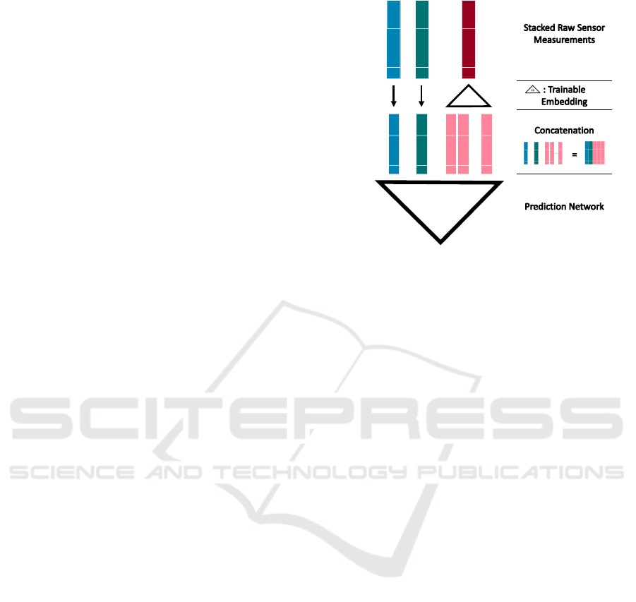
3.5 The Method

In our method, the Triplet-Stream is processed by

DNNs, which are capable to process variable fea-

ture spaces. For this, the modality indicators need to

be encoded. The categories of the analyzed datasets

are ﬁnite, mutually exclusive and known a-priori.

Due to the disadvantages of Constant Encoding al-

gorithms, we choose the Word-Embedding approach

introduced by (Guo and Berkhahn, 2016), cf. Section

3.4. Thereby, the embedding size can be considered

as further hyperparameter.

The method we propose is shown in Figure 4.

It can be seen that the modality indicators are pro-

cessed by the trainable Embedding-Network in ad-

vance. Subsequently, the encoded categories are con-

catenated with the original time and value informa-

tion. The combined representation is then processed

by the prediction network. To identify, which DNN

architecture is best suited as Prediction Head, cf. Fig-

ure 4, we evaluate the GRU network designed by (Cho

et al., 2014) and the InceptionTime network designed

Time Value

…

Prediction

Head

Figure 4: The generic Deep Neural Network (DNN)-

Architecture for MaTS.

by (Fawaz et al., 2020). The GRU-based approach

is referred to as GRU-Triplet-Stream (GRUTS) and

the InceptionTime-based approach is referred to as

InceptionTime-Triplet-Stream (ITTS).

GRU based models have shown promising results

applied on MaTS datasets (Che et al., 2018). In con-

trast, the performance of the InceptionTime network

applied to MaTS datasets has barely been studied.

The InceptionTime network is designed modular with

the help of blocks. To overcome the vanishing gra-

dient problem residual connections are used. Each

block consists of a dimension-reducing bottleneck

layer and convolution layers with different kernel-

sizes. The different kernel-sizes generate a broader

and improved ﬁeld-of-vision. Subsequently, the out-

puts of the convolution layers are concatenated with

the output of a MaxPool layer, which is applied to

the input of the block. Following the last inception

block a global average pooling is applied to generate

a ﬁxed dimensional space which is forwarded to a lin-

ear layer. The amount of blocks, the size of kernels

but also the amount of bottleneck channels are impor-

tant hyperparameters of the model.

4 EXPERIMENT

In the experiments we evaluated the GRUTS and the

ITTS on two irregular sampled and asynchronous

multivariate time series datasets: The ﬁrst one is a bi-

nary classiﬁcation task based on the PhysioNet-2012

dataset and the second one is a regression task based

on the Vehicle Engine Component Aging (VECA)

dataset.

Data Streams: Investigating Data Structures for Multivariate Asynchronous Time Series Prediction Problems

691

4.1 Datasets

The PhysioNet-2012 Challenge dataset contains

12000 Intensive Care Unit (ICU) admissions (Gold-

berger et al., 2000; Silva et al., 2012). At the be-

ginning, only 4000 ICU admissions possessed labels

(named as Set-a). The dataset was extended over the

past few years, which results in currently ∼ 12000 la-

beled ICU admissions. Each patient was admitted to

one of a variety of ICUs for e.g. medical, trauma and

surgical reasons. The ICU stay of the patient needed

to last at least 48 hours, otherwise the patients have

been excluded from the dataset. The dataset contains

41 variables of which ﬁve generic descriptors are only

measured once such as the age and the weight of the

patient. The remainder of 36 variables represents time

series with multiple observations. Each observation

got a time stamp which describes the time, which has

passed since the initial admission of the individual pa-

tient. Five outcome descriptors are available in the

dataset such as length of stay or length of survival.

Within this study we focused on the in-hospital mor-

tality (1:=died; 0:=survived). This led to a dataset,

which is strongly imbalanced. Less than 15% of the

labeled ICU stays are positive.

To be comparable to the work of (Rubanova et al.,

2019; Shukla and Marlin, 2021), we chose the Set-

a with 4000 labeled patients as the ﬁrst benchmark

dataset. We refer to this as PhysioNet-a dataset. To

further be comparable to the work of (Horn et al.,

2020), we created a second benchmark dataset from

the whole 12000 labeled patients and applied the

same train-test-split as (Horn et al., 2020). We refer

to this as PhysioNet-b dataset.

The Vehicle Engine Component Aging dataset has

been introduced by (Sass et al., 2019). The com-

ponent under investigation was the Exhaust Gas Re-

circulation (EGR) cooling system. The EGR system

is used in diesel engines to regulate the combustion

temperature within the combustion chamber. The ag-

ing represents the degree of pollution of the EGR-

cooler. The investigated degree of aging of the pro-

totype in the development stage is detected in service

intervals by measuring the fresh air mass ﬂow once

with enabled EGR-system ˙m

open

and once with dis-

abled EGR-system ˙m

closed

. The aging over time is

then deﬁned as mass ﬂow ratio ˙m

= ˙m

open

/ ˙m

closed

While utilizing interpolation, the aging in the range

of (0, 1) is continuously deﬁned over the whole inves-

tigated time span.

The corresponding vehicle data are one dimen-

sional in-vehicle sensor information recorded within

the time of component aging. With respect to the

investigation of (Sass et al., 2020), who identiﬁed

and classiﬁed the importance of sensors to monitor

the aging, we selected the seven most relevant sen-

sors. Based on the properties of the underlying bus-

network, the multivariate time series space is asyn-

chronous as asynchronicity has been deﬁned in Sec-

tion 1. Furthermore, we increased the effect of asyn-

chronicity and reduced the size of the MaTS space

to 49.16 % of the original allocated size with the use

of the Binary Shift Compression (BiSCo) algorithm

(lossless conﬁguration) introduced by (Vox et al.,

2022).

The total component aging dataset contains seven

unevenly spaced time series as features and one la-

bel time series, which describes the aging. In total,

the encoded dataset is deﬁned by 29.883.593 obser-

vations over the multivariate time series space. How-

ever, the technical requirement of a minute-by-minute

prediction of component aging leads to 38.426 la-

beled samples which we created with a sliding win-

dow approach. Furthermore, we took the last aging

information within the window to label the sample.

4.2 Competitors

As competitors we have chosen models which have

shown suitable properties to process asynchronous

vehicle sensor data. These models are listed below:

• The Phased-LSTM model (Neil et al., 2016)

• The GRU-D model (Che et al., 2018)

• The L-ODE-ODE model (Rubanova et al., 2019)

• The IPNet model (Shukla and Marlin, 2019)

• The SeFT model (Horn et al., 2020)

• The mTAND model (Shukla and Marlin, 2021)

All models are described in detail in Section 2.

4.3 Experimental Setup

All experiments have been written in the program-

ming language Python, where we used the PyTorch

and the Tensorﬂow framework (Abadi et al., 2016;

Paszke et al., 2019). All experiments are executed

with a GPU of type NVIDIA Tesla K80, which

has access to 6 cores and 56 GB of RAM. Further-

more, we used the Adam optimizer during learn-

ing phase for all Triplet-Stream experiments (Kingma

and Ba, 2015). To ﬁnd the best hyperparameter

conﬁguration for the problems under investigation

we used a Bayesian optimization approach called

Heteroscedastic Evolutionary Bayesian Optimisation

(HEBO) (Cowen-Rivers et al., 2022). HEBO has

shown outstanding performance on a benchmark

ICPRAM 2023 - 12th International Conference on Pattern Recognition Applications and Methods

692

dataset compared to other hyperparameter optimiza-

tion algorithms (Turner et al., 2021). For repro-

ducibility, the best hyperparameters of the individual

models for the two benchmark datasets are presented

in the APPENDIX.

4.4 Classiﬁcation Results

Due to the imbalanced PhysioNet datasets

(PhysioNet-a and PhysioNet-b) we used the Area

Under the Receiver Operating Characteristic

Curve (AUROC) score instead of the binary accuracy

to compare the classiﬁcation performance. The ITTS

and the GRUTS model have been trained with the

cross-entropy loss. Thereby, we applied a mini-batch

stochastic training approach. Also, we evaluated the

classiﬁcation performance of the test dataset for each

epoch. Through an extensive hyperparameter search

we identiﬁed the best model conﬁgurations and

simulated them ten times, for which the performance

(mean and standard deviation) is shown in Table 1.

The best model conﬁgurations are listed in Table 4

and 5 in the APPENDIX. It can be seen from the

Table 1: Visualization of the classiﬁcation performance for

medical health prediction problems.

Model AUROC

PhysioNet-a PhysioNet-b

GRU-D 0.818 ± 0.008

0.863 ± 0.003

†

Phased-LSTM 0.836 ± 0.003

0.790 ± 0.010

†

IPNet 0.819 ± 0.006

0.860 ± 0.002

†

SeFT 0.795 ± 0.015

0.851 ± 0.004

†

L-ODE-ODE 0.829 ± 0.004

0.857 ± 0.006

†

mTAND 0.854 ± 0.001

ITTS 0.801 ± 0.014 0.828 ±0.003

GRUTS 0.834 ± 0.004 0.857 ± 0.002

Published by (Shukla and Marlin, 2021)

†

Published by (Horn et al., 2020)

table that the mTAND model reached the highest

classiﬁcation performance for the PhysioNet-a

dataset. It is worth noting that we were not able to

reproduce the published accuracy of the mTAND

model, which deviated in our experiments by ap-

proximately two percentage points to 0.83. For the

PhysioNet-b dataset the GRU-D model reached the

highest AUROC score.

From the results it can be taken that the GRUTS

approach achieved a classiﬁcation performance com-

parable to advanced attention models and compa-

rable to modiﬁed recurrent networks such as the

GRU-D. Also, for the more transparent results of the

PhysioNet-b benchmark the GRUTS model deviated

only by 0.6 percentage points, which is interesting

due to the fact that (Che et al., 2018) compared dif-

ferent GRU based methods on MaTS prediction prob-

lems and showed that their GRU-D model outper-

formed standard GRUs signiﬁcantly. Moreover, from

the results it can be taken that the ITTS approach

did not perform well on the PhysioNet classiﬁcation

benchmarks.

4.5 Regression Results

To be able to fairly compare the performance for

the VECA regression task of the individual models

a train-test-split of 80%-20% has been applied to the

VECA dataset. We excluded the L-ODE-ODE model

because of the escalating training time per epoch

caused by the ODE-solver, which made a fair com-

parison by an appropriate hyperparameter tuning im-

possible. Within the mini-batch based learning al-

gorithm we used the Mean-Squared-Error (MSE) as

loss term. All investigated models have been exten-

sively hyperparameter tuned with HEBO, where we

used the model implementations of (Horn et al., 2020)

and (Shukla and Marlin, 2021). The resulting optimal

hyperparameters are depicted in Table 6 in the AP-

PENDIX. Furthermore, the regression performance of

the best hyperparameter conﬁguration for each model

under investigation is shown in Table 2. The simula-

tion for each model has been repeated three times to

present the RMSE with mean and standard deviation.

From the results of the regression benchmark it can be

seen that the GRUTS model reached the best perfor-

mance while the ITTS model enabled a more stable

convergence based on the lower standard deviation

with a comparable RMSE as the GRUTS. Without

forcing the hyperparameter tuning algorithm to search

for small models, the model with the lowest capacity

and thus with the lowest number of trainable param-

eters is the IPNet model. If the epoch time quality

characteristic is considered, then the SeFT model is

the fastest model which we evaluated. While taking

into account the RMSE, the epoch time and the ca-

pacity holistically the most suited model to solve the

regression problem is the ITTS approach due to the

Pareto optimum of the three quality measures.

4.6 Ablation Study

Besides the model size the sample data structure and

the resulting array size in the main memory is a fur-

ther important criterion for embedded devices such as

vehicles and batch based training on graphic cards.

Hence, we investigated the amount of bytes which

have to be allocated for the data structures of Section

Data Streams: Investigating Data Structures for Multivariate Asynchronous Time Series Prediction Problems

693

Table 2: Visualization of the regression performance deﬁned as Root-Mean-Squared-Error (RMSE) (mean ± std), the mean

epoch time in seconds and the model capacity deﬁned as trainable parameters. The RMSE evaluation metric was multiplied

by 1000 to improve readability.

Model RMSE Capacity Epoch Time

Model

Impl.

Phased-LSTM 1.736 ± 0.337 482,305 6395.84 (Horn et al., 2020)

GRU-D 3.214 ± 0.598 49,695 6740.68 (Horn et al., 2020)

IPNet 3.304 ± 0.510 15,057 2095.66 (Horn et al., 2020)

SeFT 2.933 ± 0.817 122,033 56.88 (Horn et al., 2020)

mTAND 3.367 ± 1.228 105,733 1886.58 (Shukla and Marlin, 2021)

†

ITTS 1.301 ± 0.082 82,094 138.11 cf. Section 3.5

†

GRUTS 1.250 ± 0.450 108,064 437.80 cf. Section 3.5

†

Tensorﬂow v2.9.1;

†

PyTorch v1.12

In Table 3 the data structures are linked to the

model implementations. Moreover, the table shows

the mean sample size in Bytes of 30 randomly se-

lected samples of the VECA dataset. It can be seen

that the interpolation based data structure (a

) results

in a sample size which is by a factor of 1000 bigger

than the other data structures. To ensure that each sen-

sor information is represented without loss of infor-

mation, we used an interpolation frequency of 10 Hz.

Likewise, the standard deviation of the interpolated

data structure is noteworthy because a few of the sam-

ples allocated more than 1 GB. Thus, the interpolated

data structure is rather inappropriate. The mean value

imputed data structure is approximately 50% smaller

than the masked data structure, which is caused by

the additional mask. Also, it can be taken from the ta-

ble that the Triplet-Stream data structure is the second

smallest. In comparison to the masked data structure,

the Triplet-Stream reduced the needed memory space

by approximately 80%.

4.7 Discussion

In the experiments we showed that the Triplet-Stream

combined with CNN and RNN prediction heads can

compete and even outperform state-of-the-art atten-

tion and recurrent models in the domain of MaTS. We

showed that an efﬁcient data structure and a suitable

encoding of modality indicators enabled high perfor-

mance of general purpose DNNs in the classiﬁcation

task and in the regression task.

For the classiﬁcation task we used the published

results of (Shukla and Marlin, 2021), because we

were not able to reproduce them. Nevertheless, the

GRUTS approach obtained sufﬁcient performance

within the classiﬁcation benchmark. In the regression

benchmark we showed that the Triplet-Stream is an

efﬁcient method for vehicle sensor data based regres-

sion problems.

5 CONCLUSION

In this paper we elaborated a need for research for

processing MaTS in DNNs. Therefore, we devel-

oped the Triplet-Stream, which is a lightweight data-

structure without missingness indicators or value im-

putation strategies. Thus, we did not change the raw

sensor data distribution, to minimize data based bias.

We combined the Triplet-Stream with an embedding

stage and a subsequent prediction head. As prediction

heads we evaluated the GRU model and the Incep-

tionTime model. The GRUTS and the ITTS as well

as other relevant models were benchmarked on a re-

gression problem and on a classiﬁcation problem.

The evaluation has shown that the GRUTS model

achieved excellent performance on the classiﬁcation

problem. Furthermore, the Triplet-Stream based

models outperformed existing state-of-the-art models

on the regression dataset. The ITTS model achieved

Pareto-optimal results regarding the quality measures

accuracy, training time per epoch, model capacity and

sample size. Consequently, we demonstrated an ap-

propriateness of our method to enable a sustainable

application of deep learning. Based on these results,

the Triplet-Stream approach should further be stud-

ied and analyzed on different multivariate time series

based prediction problems.

In future work, we will continue the investigation

of suitable data structures for DNNs. We will evaluate

their impact on the model size for vehicle sensor data

based prediction problems. Also, we will study the

impact of processing synchronous time series with the

Triplet-Stream and compare the results to the standard

approach. Likewise, we will extend the investigation

to vehicle ﬂeets and analyze the energy demand of

DNNs. Through this, we want to evaluate the energy

consumption of models when they are fully deployed.

ICPRAM 2023 - 12th International Conference on Pattern Recognition Applications and Methods

694

Table 3: Combining the data structures of Figure 2 and Figure 3 with the models under investigation and the resulting VECA

sample size.

Data Structure Sample Size in Byte Model

Interpolated (a

) 4.017e8 ± 1.060e9 -

Imputed (a

) 4.591e4 ± 3.647e4 -

Masked (b) 8.608e4 ± 7.837e4

SeFT, IPNet, mTAND

GRU-D, Phased-LSTM

Raw (c) 1.148e4 ± 9.116e3 -

Triplet-Stream 1.722e4 ± 1.367e4 GRUTS, ITTS

DISCLAIMER

The results, opinions, and conclusions expressed in

this publication are not necessarily those of Volkswa-

gen Aktiengesellschaft.

REFERENCES

Abadi, M., Barham, P., Chen, J., Chen, Z., Davis, A., Dean,

J., Devin, M., Ghemawat, S., Irving, G., Isard, M.,

et al. (2016). Tensorﬂow: A system for large-scale

machine learning. In 12th USENIX Symposium on

Operating Systems Design and Implementation (OSDI

16), pages 265–283.

Cerda, P. and Varoquaux, G. (2022). Encoding high-

cardinality string categorical variables. IEEE

Transactions on Knowledge and Data Engineering,

34(3):1164–1176.

Cerda, P., Varoquaux, G., and K

egl, B. (2018). Similarity

encoding for learning with dirty categorical variables.

Machine Learning, 107(8-10):1477–1494.

Che, Z., Purushotham, S., Cho, K., Sontag, D., and Liu,

Y. (2018). Recurrent neural networks for multivari-

ate time series with missing values. Scientiﬁc reports,

8(1):6085.

Cho, K., van Merrienboer, B., Gulcehre, C., Bahdanau, D.,

Bougares, F., Schwenk, H., and Bengio, Y. (2014).

Learning phrase representations using rnn encoder–

decoder for statistical machine translation. Proceed-

ings of the 2014 Conference on Empirical Methods in

Natural Language Processing, EMNLP, pages 1724–

1734.

Cowen-Rivers, A. I., Lyu, W., Tutunov, R., Wang, Z.,

Grosnit, A., Grifﬁths, R. R., Maraval, A. M., Jianye,

H., Wang, J., and Peters, J. (2022). Hebo: push-

ing the limits of sample-efﬁcient hyper-parameter op-

timisation. Journal of Artiﬁcial Intelligence Research,

74:1269–1349.

Fawaz, H. I., Lucas, B., Forestier, G., Pelletier, C., Schmidt,

D. F., Weber, J., Webb, G. I., Idoumghar, L., Muller,

P.-A., and Petitjean, F. (2020). Inceptiontime: Finding

alexnet for time series classiﬁcation. Data Mining and

Knowledge Discovery, 34(6):1936–1962.

Futoma, J., Hariharan, S., and Heller, K. (2017). Learn-

ing to detect sepsis with a multitask gaussian process

rnn classiﬁer. International Conference on Machine

Learning, ICML, 34:1174–1182.

Goldberger, A. L., Amaral, L. A. N., Glass, L., Hausdorff,

J. M., Ivanov, P. C., Mark, R. G., Mietus, J. E., Moody,

G. B., Peng, C.-K., and Stanley, H. E. (2000). Phys-

iobank, physiotoolkit, and physionet: Components of

a new research resource for complex physiologic sig-

nals. Circulation, 101(23):215–220.

Guo, C. and Berkhahn, F. (2016). Entity embeddings of cat-

egorical variables. arXiv preprint arXiv:1604.06737.

Hewamalage, H., Bergmeir, C., and Bandara, K. (2021).

Recurrent neural networks for time series forecast-

ing: Current status and future directions. International

Journal of Forecasting, 37(1):388–427.

Hochreiter, S. and Schmidhuber, J. (1997). Long short-term

memory. Neural computation, 9(8):1735–1780.

Horn, M., Moor, M., Bock, C., Rieck, B., and Borgwardt,

K. (2020). Set functions for time series. International

Conference on Machine Learning, ICML, 37:4353–

4363.

Kingma, D. P. and Ba, J. (2015). Adam: A method for

stochastic optimization. International Conference on

Learning Representations, ICLR, 3.

Li, S. C.-X. and Marlin, B. (2016). A scalable end-to-

end gaussian process adapter for irregularly sampled

time series classiﬁcation. International Conference

on Neural Information Processing Systems, 30:1812–

1820.

Lipton, Z., Kale, D., and Wetzel, R. (2016). Modeling miss-

ing data in clinical time series with rnn. Proceedings

of Machine Learning for Healthcare 2016.

Little, R. J. A. and Rubin, D. B. (2019). Statistical analysis

with missing data, volume 793. John Wiley & Sons.

Ma, J., Shou, Z., Zareian, A., Mansour, H., Vetro, A., and

Chang, S.-F. (2019). Cdsa: Cross-dimensional self-

attention for multivariate, geo-tagged time series im-

putation. arXiv preprint arXiv:1905.09904.

Neil, D., Pfeiffer, M., and Liu, S.-C. (2016). Phased

lstm: Accelerating recurrent network training for long

or event-based sequences. International Conference

on Neural Information Processing Systems, 30:3889–

3897.

Paszke, A., Gross, S., Massa, F., Lerer, A., Bradbury, J.,

Chanan, G., Killeen, T., Lin, Z., Gimelshein, N.,

Antiga, L., Desmaison, A., Kopf, A., Yang, E., De-

Vito, Z., Raison, M., Tejani, A., Chilamkurthy, S.,

Steiner, B., Fang, L., Bai, J., and Chintala, S. (2019).

Pytorch: An imperative style, high-performance deep

learning library. Advances in Neural Information Pro-

cessing Systems, 32:8024–8035.

Data Streams: Investigating Data Structures for Multivariate Asynchronous Time Series Prediction Problems

695

Rabiner, L. R. (1989). A tutorial on hidden markov models

and selected applications in speech recognition. Pro-

ceedings of the IEEE, 77(2):257–286.

Ramati, M. and Shahar, Y. (2010). Irregular-time bayesian

networks. Conference on Uncertainty in Artiﬁcial In-

telligence, UAI, 26.

Rasmussen, C. E. and Williams, C. K. I. (2006). Gaussian

Processes for Machine Learning. MIT Press.

Rubanova, Y., Chen, R. T. Q., and Duvenaud, D. (2019).

Latent odes for irregularly-sampled time series. Ad-

vances in Neural Information Processing Systems, 32.

Sass, Andreas Udo, Esatbeyoglu, E., and Fischer, T.

(2019). Monitoring of powertrain component aging

using in-vehicle signals. Diagnose in mechatronis-

chen Fahrzeugsystemen XIII, pages 15–28.

Sass, Andreas Udo, Esatbeyoglu, E., and Iwwerks, T.

(2020). Signal pre-selection for monitoring and pre-

diction of vehicle powertrain component aging. Pro-

ceedings of the 16th European Automotive Congress,

pages 519–524.

Schwartz, R., Dodge, J., Smith, N. A., and Etzioni, O.

(2020). Green ai. Communications of the ACM,

63(12):54–63.

Shih, S.-Y., Sun, F.-K., and Lee, H.-y. (2019). Temporal

pattern attention for multivariate time series forecast-

ing. Machine Learning, 108(8-9):1421–1441.

Shukla, S. and Marlin, B. (2019). Interpolation-prediction

networks for irregularly sampled time series. In-

ternational Conference on Learning Representations,

ICLR, 7.

Shukla, S. N. and Marlin, B. M. (2021). Multi-time atten-

tion networks for irregularly sampled time series. In-

ternational Conference on Learning Representations,

ICLR, 9.

Silva, I., Moody, G., Scott, D. J., Celi, L. A., and Mark,

R. G. (2012). Predicting in-hospital mortality of icu

patients: The physionet/computing in cardiology chal-

lenge 2012. In 2012 Computing in Cardiology, pages

245–248.

Song, H., Rajan, D., Thiagarajan, J. J., and Spanias, A.

(2018). Attend and diagnose: Clinical time series

analysis using attention models. Proceedings of the

AAAI conference on artiﬁcial intelligence, 32(1).

Sun, C., Hong, S., Song, M., and Li, H. (2020). A review of

deep learning methods for irregularly sampled medi-

cal time series data. arXiv preprint arXiv:2010.12493.

Szegedy, C., Vanhoucke, V., Ioffe, S., Shlens, J., and Wojna,

Z. (2016). Rethinking the inception architecture for

computer vision. Proceedings of the IEEE conference

on computer vision and pattern recognition.

Turner, R., Eriksson, D., McCourt, M., Kiili, J., Laaksonen,

E., Xu, Z., and Guyon, I. (2021). Bayesian optimiza-

tion is superior to random search for machine learn-

ing hyperparameter tuning: Analysis of the black-box

optimization challenge 2020. NeurIPS 2020 Compe-

tition and Demonstration Track, pages 3–26.

Vaswani, A., Shazeer, N., Parmar, N., Uszkoreit, J., Jones,

L., Gomez, A. N., Kaiser, L., and Polosukhin, I.

(2017). Attention is all you need. Advances in Neural

Information Processing Systems, 30.

Vox, C., Broneske, D., Piewek, J., Sass, A. U., and Saake,

G. (2022). Integer time series compression for holistic

data analytics in the context of vehicle sensor data. In

International Conference on Connected Vehicle and

Expo (ICCVE), pages 1–7.

Weerakody, P. B., Wong, K. W., Wang, G., and Ela, W.

(2021). A review of irregular time series data handling

with gated recurrent neural networks. Neurocomput-

ing, 441(7):161–178.

Wu, S., Liu, S., Sohn, S., Moon, S., Wi, C.-I., Juhn, Y.,

and Liu, H. (2018). Modeling asynchronous event se-

quences with rnns. Journal of biomedical informatics,

83:167–177.

Yang, B., Sun, S., Li, J., Lin, X., and Tian, Y. (2019). Trafﬁc

ﬂow prediction using lstm with feature enhancement.

Neurocomputing, 332(4):320–327.

Zaheer, M., Kottur, S., Ravanbakhsh, S., Poczos, B.,

Salakhutdinov, R. R., and Smola, A. J. (2017). Deep

sets. Advances in Neural Information Processing Sys-

tems, 30.

APPENDIX

Table 4: Classiﬁcation Benchmark I.

Best hyperparameters for the PhysioNet-a dataset

ITTS: n-blocks=3, bottleneck-channels=2, n-ﬁlters=12, kernel-

sizes=[4, 8, 16], activation=hardswish, out-activation=sigmoid, n-

embeddings=15, linear-hidden=[256], use-residual=True, min-max-

scaling=False; GRUTS: rnn-hidden=55, rnn-depth=5, activation=gelu,

linear-hidden=[65, 33], n-embeddings=69, min-max-scaling=False

Table 5: Classiﬁcation Benchmark II.

Best hyperparameters for the PhysioNet-b dataset

ITTS: n-blocks=1, bottleneck-channels=12, n-ﬁlters=16, kernel-

sizes=[4, 8, 16], activation=tanh, out-activation=linear, n-

embeddings=20, linear-hidden=[128], use-residual=True, min-

max-scaling=False; GRUTS: rnn-hidden=235, rnn-depth=7,

activation=tanh, linear-hidden=[424], n-embeddings=176, min-

max-scaling=False

Table 6: Regression Benchmark.

Best hyperparameters for the VECA dataset

Phased-LSTM: n-units=256, use-peepholes=True, leak=0.001,

period-init-max=1000.0; GRU-D: n-units=120, dropout=0.0,

recurrent-dropout=0.01; IPNet: n-units=60, dropout=0.0, recurrent-

dropout=0.1, imputation-stepsize=1.0, reconst-fraction=0.01; SeFT:

n-phi-layers=1, phi-width=165, phi-dropout=0.0, n-psi-layers=3,

psi-width=28, psi-latent-width=121, dot-prod-dim=90, n-heads=7,

attn-dropout=0.1, latent-width=40, n-rho-layers=4, rho-width=24, rho-

dropout=0.0, n-positional-dims=4, max-timescale=100.0; mTAND:

query-steps=196, rec-hidden=94, embed-time=88, num-heads=4,

freq=9, learn-emb=True, regressor-layer-size=134; ITTS: n-

blocks=6, bottleneck-channels=2, n-ﬁlters=13, kernel-sizes=[4,

32, 128], activation=relu, out-activation=sigmoid, n-embeddings=1,

linear-hidden=[256], use-residual=True, min-max-scaling=True;

GRUTS: rnn-hidden=64, rnn-depth=5, activation=hardswish, linear-

hidden=[128, 64, 32, 16], n-embeddings=1, min-max-scaling=True

ICPRAM 2023 - 12th International Conference on Pattern Recognition Applications and Methods

696