Modified kNN Classifier in the Output Vector Space for Robust
Performance Against Adversarial Attack
C. Lee, D. Seok, D. Shim and R. Park
Dept. of Electronical and Electronic Engineering, Yonsei University, Republic of Korea
Keywords: CNN-Based Classifier, Modified kNN Classifier, Adversarial Attack, Output Vector Space.
Abstract: Although CNN-based classifiers have been successfully applied to many pattern classification problems, they
suffer from adversarial attacks. Slightly modified images can be classified as completely different classes. It
has been reported that CNN-based classifiers tend to construct decision boundaries close to training samples.
In order to mitigate this problem, we applied modified kNN classifiers in the output vector space of CNN-
based classifiers. Experimental results show that the proposed method noticeably reduced the classification
error caused by adversarial attacks.
1 INTRODUCTION
CNN-based classifiers have been applied in various
pattern recognition and signal/image processing areas,
which include object recognition (Barbu, 2019;
Hendrycks, 2021; Wang, 2019; Ouyang, 2015, Wonja,
2017, Girshick, 2014), image processing (Jin, 2017;
Kim, 2021), speech recognition (Sainath, 2015,
Amodei, 2016), medical imaging (Gibson, 2018), and
super-resolution (Kim, 2017; Lee, 2021). Although
they produced good performance compared to
conventional methods, CNN-based classifiers have a
reliability problem. One can easily make a CNN-
based classifier to misclassify slightly modified
images (Szegedy, 2014). For example, Fig. 1(a) is
correctly classified as ‘4’ while Fig. 1(b) is
misclassified as ‘8’. The vulnerability of CNN-based
classifiers to this kind of adversarial attack is a serious
reliability issue, which is still unsolved (Goodfellow,
2015; Ilyas, 2019; Akhtar, 2018).
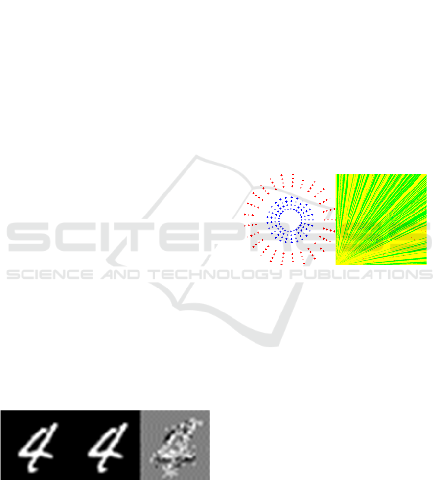
Figure 1: (a) Correctly classified image, (b) adversarial
example misclassified as 8, (c) magnified difference image.
It has been reported (Woo, 2018) that CNN-based
classifiers tend to construct decision boundaries close
(a) (b)
Figure 2: Decision boundary formation of neural networks
for circular distributions. (a) Circular distribution of two
classes, (b) decision boundaries.
to training samples (Fig. 2). In particular, when the
ReLU function is used, it appears that the decision
boundaries failed to construct desirable decision
boundaries that divide the input space into
meaningful subregions even in a low dimensional
space. Even when the sigmoid function was used as
activation functions, the results were not very
promising (Woo, 2018). If the training samples
contain some erroneous samples, which may almost
always happen in a real-world application, the neural
networks with the sigmoid function also failed to
construct proper decision boundaries.
In order to reduce this kind of vulnerability of
CNN-based classifiers, we evaluated a modified kNN
classifier in the output vector space of CNN-based
classifiers. The output vector space is the last layer of
CNN structures and the dimension is the same as the
number of classes. The number of training samples to
train a CNN-based classifier can be very large. For
Lee, C., Seok, D., Shim, D. and Park, R.
Modified kNN Classifier in the Output Vector Space for Robust Performance Against Adversarial Attack.
DOI: 10.5220/0011735800003411
In Proceedings of the 12th International Conference on Pattern Recognition Applications and Methods (ICPRAM 2023), pages 443-449
ISBN: 978-989-758-626-2; ISSN: 2184-4313
Copyright
c
 2023 by SCITEPRESS – Science and Technology Publications, Lda. Under CC license (CC BY-NC-ND 4.0)
443

example, for the ImageNet database, the number of
training samples is 1281167. In the conventional kNN
classifier, we need to compute the distances between a
test sample and all the training samples. Consequently,
the computational cost can be prohibitively large. In
order to solve this problem, we propose a modified
kNN classifier for the classification in the output vector
space. To evaluate the proposed method, we applied
the modified kNN classifier to 12 CNN-based
classifiers (Simonyan, 2014; Zhang, 2016; Zagoruyko,
2016; Simonyan, 2015; Huang, 2017; Sandler, 2018;
Xie, 2017; Szegedy, 2015; Szegedy, 2016; Ma, 2018;
Tan, 2019).
2 ADVERSARIAL IMAGES
It has been reported that one can easily fool a CNN-
based classifier by slightly modifying images so that
the classifier would misclassify the modified images.
Almost all CNN-based classifiers are vulnerable to
adversarial attacks. We generated adversarial images
of 12 CNN-based classifiers for correctly classified
validation samples of the ImageNet database. The
difference between an adversarial image and the
corresponding original image can be defined as
follows:
ori adv
DI I=−
where
ori
I
is an original image after normalization
and
adv
I
is an adversarial image. We generated
adversarial images of various distances (D=1, 2, 4, 8,
16, 32). Figs. 3-8 show some adversarial images of
the various distances. In particular, as can be seen in
Fig. 9 (D=1), some adversarial images are
indistinguishable from the original images. Most of
the adversarial class images have some similar
features and these results indicate that the current
CNN-based classifiers form decision boundaries very
close to training samples. Several observations can
be made about the adversarial images. Some
adversarial image classes have similar characteristics
whereas others appear to be completely different. As
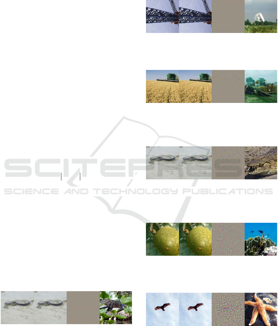
(a) (b) (c) (d)
Figure 3: Class C65 (sea snake) is misclassified as C50
(American alligator, Alligator mississipiensis). (a) original,
(b) adversarial, (c) difference (D=1), (d) representative
image of C50.
the distance increase, some artifacts become visible
and it is more likely that the adversarial images are
misclassified as completely unlikely classes.
(a) (b) (c) (d)
Figure 4: Class C517 (crane) is misclassified as C755 (radio
telescope, radio reflector). (a) original, (b) adversarial, (c)
difference (D=2), (d) representative image of C755.
(a) (b) (c) (d)
Figure 5: Class C595 (harvester, reaper) is misclassified as
C856 (thresher, thrasher, threshing machine). (a) original,
(b) adversarial, (c) difference (D=4), (d) representative
image of C856.
(a) (b) (c) (d)
Figure 6: Class C65 (sea snake) is misclassified as C49
(African crocodile, Nile crocodile, Crocodylus niloticus).
(a) original, (b) adversarial, (c) difference (D=8), (d)
representative image of C49.
(a) (b) (c) (d)
Figure 7: Class C109 (brain coral) is misclassified as C973
(coral reef). (a) original, (b) adversarial, (c) difference
(D=16), (d) representative image of C973.
(a) (b) (c) (d)
Figure 8: Class C23 (vulture) is misclassified as C327
(starfish, sea star). (a) original, (b) adversarial, (c)
difference (D=32), (d) representative image of C327.
ICPRAM 2023 - 12th International Conference on Pattern Recognition Applications and Methods
444

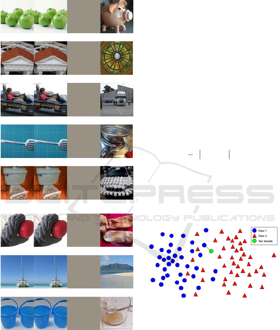
C948(Granny Smith)→C719(piggy bank, penny bank)
C858(tile roof) → C538(dome)
C573(go-kart) → C561(forklift)
C813(spatula)→ C784(screwdriver)
C861(toilet seat) → C999(toilet tissue, toilet paper, bathroom
tissue)
C658(mitten) → C911(wool, woolen, woollen)
C484(catamaran) → C977(sandbar, sand bar)
C463(bucket, pail) → C647(measuring cup)
Figure 9: Indistinguishable adversarial images with very
small differences (D=1). The first column images are
original images, the second column images are adversarial
images, the third column images are difference images, and
the fourth column images are representative images of the
adversarial classes.
3 MODIFIED KNN CLASSIFIERS
In the conventional kNN classifier, we find the k
nearest neighbour samples of a test sample and count
the number of samples of each class (Fig. 10). Then,
we decide the class that has the largest number of
samples among the k nearest neighbour samples:
() ()
() .
ii j
ii
Decide X if g X g X
where g X k
ω ∈>
=
However, it is not easy to use the kNN classfier when
the number of training samples is very large as in the
case of the ImageNet database.
In order to solve this problem, we modified the
kNN classifier. For each test sample, we choose k top-
ranking classes. For each chosen top-ranking class of
the k classes, we find m samples closest to the test
sample. Then, we compute the average distance as
follows:
1
1
1,...,
m
class j
class j test i th closest
i
DIIjk
m
−
=
=− =

where class j is the j-th ranking class for the test
sample. Finally, we choose the class with the
minimum average distance. Using this modified kNN
classifier, we only need to compute the distances of
the test samples and kxL training samples where L is
the average number of training samples of each class.
In case of the ImageNet database, the value of L is
about 1281.
Figure 10: kNN classifier (1NN).
4 EXPERIMENTAL RESULTS
We generated adversarial images of various distances
(1, 2, 4, 8, 16, 32) using the 12 models (MnasNet,
VGG, DenseNet, MobileNet, Inception, GoogleNet,
ShuffleNet, ResNext, WideResNet, ResNet50,
ResNet101, ResNet152). The adversarial images of
all the models are very similar to the original images
when the distances are small and all the models
Modified kNN Classifier in the Output Vector Space for Robust Performance Against Adversarial Attack
445

showed similar characteristics in that such adversarial
images can be easily generated.
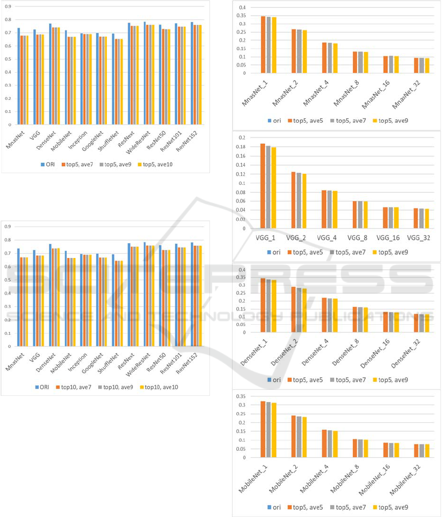
Figure 11: Performance comparison of modified kNN
classifiers. Top 5 classes were chosen and the average
values of 7, 9, 10 nearest samples were used.
Figure 12: Performance comparison of modified kNN
classifiers. Top 10 classes were chosen and the average
values of 7, 9, 10 nearest samples were used.
Fig. 11 shows a performance comparison of modified
kNN classifiers (top 5 classes were chosen and the
average values of 7, 9, 10 nearest samples were used).
Fig. 12 shows a performance comparison of modified
kNN classifiers (top 10 classes were chosen and the
average values of 7, 9, 10 nearest samples were used).
It can be seen that using top 10 classes or top 5 classes
produced very similar performance. Thus, we used
top 5 classes to classify the adversarial images.
Compared to the conventional CNN-based classifiers,
the modified kNN classifiers produced slightly lower
performance (errors increased by about 3-4% as can
be seen in Figs. 11-12).
Figure 13: Performance comparison of modified kNN
classifiers against adversarial images (MnasNet, VGG,
DenseNet, MobileNet). The original CNN-based classifiers
misclassified all the adversarial images.
ICPRAM 2023 - 12th International Conference on Pattern Recognition Applications and Methods
446

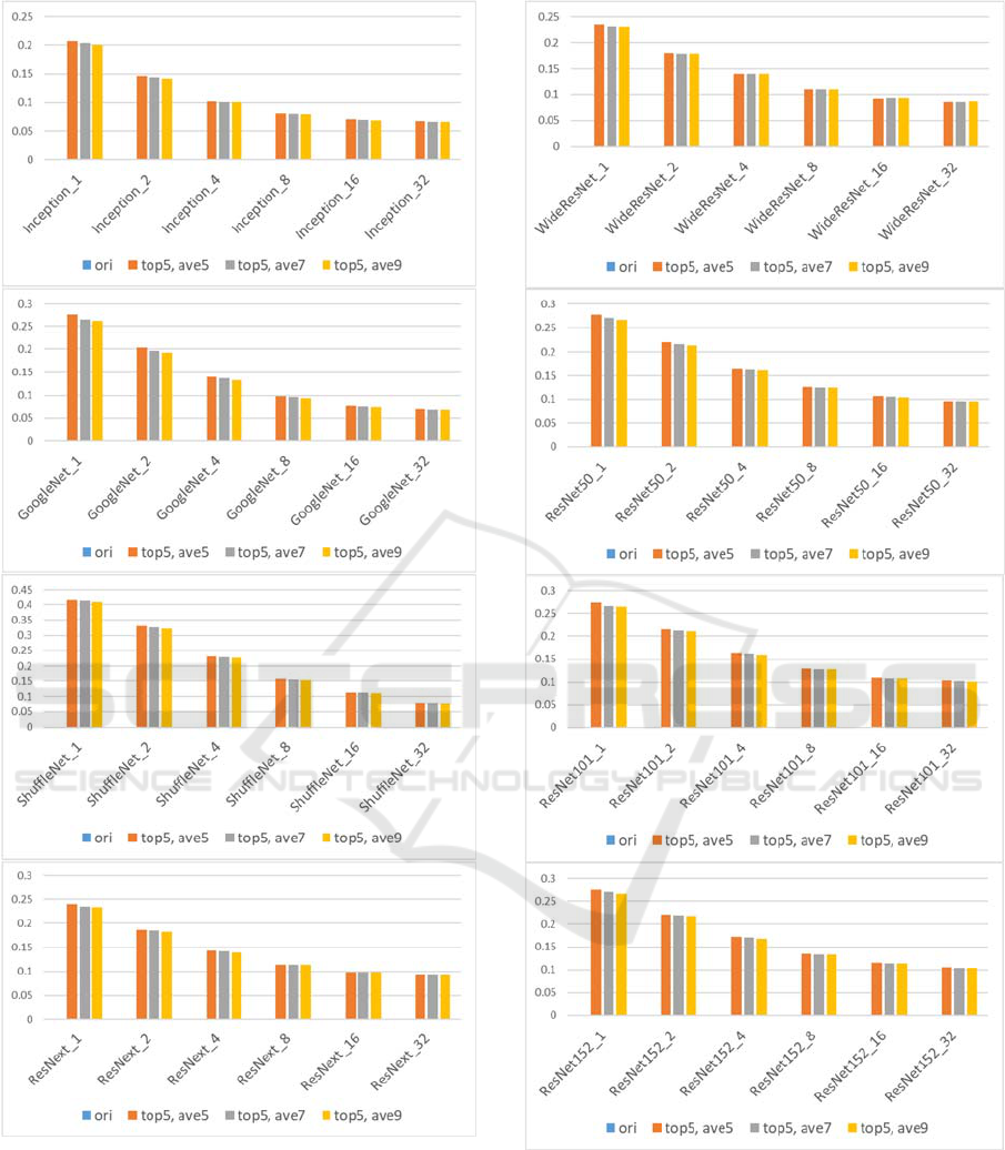
Figure 14: Performance comparison of modified kNN
classifiers against adversarial images (Inception,
GoogleNet, ShuffleNet, ResNext). The original CNN-
based classifiers misclassified all the adversarial images.
In Figs. 13-15, top 5 classes were chosen and the
average values of 5, 7, 9 nearest samples were used
for the modified kNN classifier. The original CNN-
based classifiers misclassified all the adversarial
images as expected.
Figure: 15: Performance comparison of modified kNN
classifiers against adversarial images (WideResNet,
ResNet50, ResNet101, ResNet152). The original CNN-
based classifiers misclassified all the adversarial images.
For images with small distances (D=1, 2), the
classification accuracy of the proposed kNN
classifiers is 0.187~0.415 (D=1) and 0.125~0.329
(D=2). For images with large distances (D=1, 2), the
Modified kNN Classifier in the Output Vector Space for Robust Performance Against Adversarial Attack
447

classification accuracy of the proposed method is
0.046~0.129 (D=16) and 0.044~0.116 (D=32). It is
noted that the classification accuracy of the original
CNN-based classifiers is zero (100% error) for the
adversarial images.
5 CONCLUSIONS
In this paper, we proposed modified kNN classifiers
for the output vector space of CNN-based classifiers
to provide robust performance against adversarial
attacks. To reduce the complexity problem of
conventional kNN classifiers when the number of
training samples is very large, we propose a modified
kNN classifier for CNN-based classifiers. The
proposed method was evaluated using 12 models and
showed noticeable improvement in reducing the
classification error caused by adversarial attacks. By
applying the kNN classifier in the middle layers, it
may be possible to further improve performance.
ACKNOWLEDGEMENTS
This research was supported in part by Basic Science
Research Program through the National Research
Foundation of Korea (NRF) funded by the Ministry
of Education, Science and Technology (NRF-
2020R1A2C1012221).
REFERENCES
Akhtar, Naveed and Ajmal Mian (2018). “Threat of
Adversarial Attacks on Deep Learning in Computer
Vision: A Survey,” IEEE Access.
Amodei, D., et al. (2016, June). Deep speech 2: End-to-end
speech recognition in English and Mandarin. In
International conference on machine learning (pp. 173-
182).
Barbu, A. et al. (2019). “Objectnet: A large-scale bias-
controlled dataset for pushing the limits of object
recognition models,” in Proc. Adv. Neural Inf. Process.
Syst., pp. 9448–9458.
Gibson, E., et al. (2018). NiftyNet: a deep-learning platform
for medical imaging. Computer methods and programs
in biomedicine, 158, 113-122.
Girshick, R., et al. (2014). Rich feature hierarchies for
accurate object detection and semantic segmentation. In
Proceedings of the IEEE conference on computer vision
and pattern recognition (pp. 580-587).
Goodfellow, I. J., J. Shlens, and C. Szegedy (2015).
“Explaining and harnessing adversarial examples,” in
Proc. Int. Conf. Learn. Representations.
He, K., Zhang, X., Ren, S., & Sun, J. (2016). “Deep
Residual Learning for Image Recognition,”
Proceedings of the IEEE conference on Computer
Vision and Pattern Recognition, pp. 770-778.
Hendrycks, Dan, et al. (2021). "The many faces of
robustness: A critical analysis of out-of-distribution
generalization." Proceedings of the IEEE/CVF
International Conference on Computer Vision., pp.
8340-8349.
Huang, G., et al. (2017). “Densely connected convolutional
networks,” in Proc. IEEE Conf. Comput. Vis. Pattern
Recognit., pp. 2261–2269.
Ilyas, Andrew, et al. (2019). “Adversarial examples are not
bugs, they are features,” arXiv:1905.02175.
Jin, K. H., McCann, M. T., Froustey, E., & Unser, M.
(2017). Deep convolutional neural network for inverse
problems in imaging. IEEE Transactions on Image
Processing, 26(9), 4509-4522.
Kim, J., et al. (2020). “Analyzing Decision Polygons of
DNN-based Classification Method, in Proc.
International Conference on Informatics in Control,
Automation and Robotics.
Kim, J., et al. (2016). Accurate image super-resolution
using very deep convolutional networks. In
Proceedings of the IEEE conference on computer vision
and pattern recognition (pp. 1646-1654).
Kim, J., et al., "Reliable Perceptual Loss Computation for
GAN-Based Super-Resolution With Edge Texture
Metric," in IEEE Access, vol. 9, pp. 120127-120137,
2021, doi: 10.1109/ACCESS.2021.3108394.
Koushik, J. (2016). Understanding convolutional neural
networks. arXiv preprint arXiv:1605.09081.
Lee, C., et al. (2021). “One-to-One Mapping-like Properties
of DCN-Based Super-Resolution and its Applicability
to Real-World Images,” IEEE Access, pp. 121167 –
121183.
Lim, B., et al. (2017). Enhanced deep residual networks for
single image super-resolution. In Proceedings of the
IEEE conference on computer vision and pattern
recognition workshops (pp. 136-144).
Ma, N., et al. (2018). “ShuffleNet V2: Practical guidelines
for efficient CNN architecture design,” in Proc. Eur.
Conf. Comput. Vis., Sep., pp. 122–138.
Mallat, S. (2016). Understanding deep convolutional
networks. Philosophical Transactions of the Royal
Society A: Mathematical, Physical and Engineering
Sciences, 374(2065), 20150203.
Ouyang, W., et al. (2015). Deepid-net: Deformable deep
convolutional neural networks for object detection. In
Proceedings of the IEEE conference on computer vision
and pattern recognition (pp. 2403-2412).
Radford, A., et al. (2015). Unsupervised representation
learning with deep convolutional generative adversarial
networks. arXiv preprint arXiv:1511.06434.
Sainath, T. N., et al. (2015). Deep convolutional neural
networks for large-scale speech tasks. Neural
Networks, 64, 39-48.
Sandler, M., et al. (2018). “MobileNetV2: Inverted
residuals and linear bottlenecks,” in Proc. IEEE Conf.
Comput. Vision Pattern Recognit., pp. 4510–4520
ICPRAM 2023 - 12th International Conference on Pattern Recognition Applications and Methods
448

Simonyan, K. and A. Zisserman (2015). “Very deep
convolutional networks for large-scale image
recognition,” in Proc. Int. Conf. Learn.
Representations.
Simonyan, Karen, Andrew Zisserman (2014). “Very Deep
Convolutional Networks for Large-Scale Image
Recognition,” https://doi.org/10.48550/arXiv.1409.
1556.
Szegedy, C., et al. (2016). “Rethinking the inception
architecture for computer vision,” in Proc. CVPR, pp.
2818–2826.
Szegedy, C., et al. (2015). “Going deeper with
convolutions,” in Proc. IEEE Conf. Comput. Vis.
Pattern Recognition, pp. 1–9.
Szegedy, et al. (2013). Intriguing properties of neural
networks. arXiv preprint arXiv:1312.6199.
Szegedy, Christian, et al. (2014). “Intriguing properties of
neural networks,” in Proc. International Conference on
Learning Representations.
Tan, M., et al. (2019). “MnasNet: Platform-aware neural
architecture search for mobile,” in Proc. IEEE Conf.
Comput. Vis. Pattern Recognit., pp. 2820–2828.
Wang, Haohan et al. (2019). “Learning Robust Global
Representations by Penalizing Local Predictive
Power,” Advances in Neural Information Processing
Systems, pp. 10506-10518.
Wang, X., et al. (2018). Esrgan: Enhanced super-resolution
generative adversarial networks. In Proceedings of the
European Conference on Computer Vision (ECCV)
(pp. 0-0).
Wojna, Z., et al. (2017, November). Attention-based
extraction of structured information from street view
imagery. In 2017 14th IAPR International Conference
on Document Analysis and Recognition (ICDAR) (Vol.
1, pp. 844-850).
Woo, S., et. al (2018). Decision boundary formation of deep
convolution networks with ReLU. In Intl Conf.
(DASC/PiCom/DataCom/CyberSciTech) (pp. 885-888).
Xie, S., et al. (2017). “Aggregated residual transformations
for deep neural networks,” in Proc. CVPR, pp. 5987–
5995.
Yang, H. F., et al. (2017). Supervised learning of semantics-
preserving hash via deep convolutional neural
networks. IEEE transactions on pattern analysis and
machine intelligence, 40(2), 437-451.
Yosinski, et al. (2014). How transferable are features in
deep neural networks?. In Advances in neural
information processing systems (pp. 3320-3328).
Yosinski, J., et al. (2015). Understanding neural networks
through deep visualization. arXiv preprint
arXiv:1506.06579.
Zagoruyko, S. et al. (2016). “Wide residual networks,” in
Proc. Brit. Mach. Vis. Conf., pp. 87.1–87.12.
Zeiler, M. D., & Fergus, R. (2014, September). Visualizing
and understanding convolutional networks. In
European conference on computer vision (pp. 818-
833). Springer, Cham.
Zhang, Y., et al. (2018). Image super-resolution using very
deep residual channel attention networks. In
Proceedings of the European Conference on Computer
Vision (ECCV) (pp. 286-301).
Modified kNN Classifier in the Output Vector Space for Robust Performance Against Adversarial Attack
449