The Effect of Covariate Shift and Network Training on

Out-of-Distribution Detection

Simon Mariani

, Sander R. Klomp

2 a

, Rob Romijnders

and Peter H. N. de With

2 b

University of Amsterdam, Amsterdam, The Netherlands

Eindhoven University of Technology, Eindhoven, The Netherlands

Keywords:

Out-of-Distribution Detection, Deep Learning, Convolutional Neural Networks.

Abstract:

The ﬁeld of Out-of-Distribution (OOD) detection aims to separate OOD data from in-distribution (ID) data in

order to make safe predictions. With the increasing application of Convolutional Neural Networks (CNNs) in

sensitive environments such as autonomous driving and security, this ﬁeld is bound to become indispensable

in the future. Although the OOD detection ﬁeld has made some progress in recent years, a fundamental

understanding of the underlying phenomena enabling the separation of datasets remains lacking. We ﬁnd that

the OOD detection relies heavily on the covariate shift of the data and not so much on the semantic shift, i.e.

a CNN does not carry explicit semantic information and relies solely on differences in features. Although

these features can be affected by the underlying semantics, this relation does not seem strong enough to rely

on. Conversely, we found that since the CNN training setup determines what features are learned, that it is

an important factor for the OOD performance. We found that variations in the model training can lead to an

increase or decrease in the OOD detection performance. Through this insight, we obtain an increase in OOD

detection performance on the common OOD detection benchmarks by changing the training procedure and

using the simple Maximum Softmax Probability (MSP) model introduced by (Hendrycks and Gimpel, 2016).

We hope to inspire others to look more closely into the fundamental principles underlying the separation of

two datasets. The code for reproducing our results can be found at https://github.com/SimonMariani/OOD-

detection.

1 INTRODUCTION

Although Convolutional Neural Networks (CNNs)

achieve good performance on many different tasks,

their deployment in sensitive environments does not

come without problems. In order to use CNNs safely

in tasks for self driving cars (Vojir et al., 2021; Boone

et al., 2022), medical image analysis (Mehrtash et al.,

2020; Raghu et al., 2019) or face recognition (Chang

et al., 2020; Betta et al., 2011), some degree of cer-

tainty must be given to the predictions of such a net-

work, as a misclassiﬁcation can be problematic. This

is often referred to as misclassiﬁcation detection and

is generally done on samples that can be seen as

drawn from the same distribution as the training data,

i.e. the In-Distribution (ID). Besides such samples

that are drawn from the ID, it can also be the case

that a sample was drawn from a different distribu-

tion. Such a sample can then be referred to as an Out-

of-Distribution (OOD) sample and is likely to affect

https://orcid.org/0000-0002-0874-4720

https://orcid.org/0000-0002-7639-7716

the output of the CNN. Therefore, the ﬁeld of OOD

detection is concerned with separating OOD sam-

ples from ID samples, as to increase the reliability of

CNNs. Although access to OOD data is generally not

available, some ID-OOD dataset pairs have emerged

and are being extensively used as the general bench-

mark (Hendrycks and Gimpel, 2016; Lee et al., 2018;

Lee et al., 2017). Succeeding work has been con-

cerned with the scalability of OOD detection methods

and propose larger benchmark datasets (Hendrycks

et al., 2019a; Huang and Li, 2021; Roady et al., 2019).

These benchmarks are currently the primary way of

comparing OOD detection methods and are vital for

the development of new OOD detection methods.

For this reason, we will also use the existing

benchmarks to measure performance and show that

detecting OOD samples relies heavily on the covari-

ate shift of the data and largely ignores actual class

differences. We do so by looking at the OOD samples

that share and do not share classes with the ID data, as

some of the commonly used benchmark dataset pairs

have some class overlap. For this purpose, we use

Mariani, S., Klomp, S., Romijnders, R. and N. de With, P.

The Effect of Covariate Shift and Network Training on Out-of-Distribution Detection.

DOI: 10.5220/0011725900003417

In Proceedings of the 18th International Joint Conference on Computer Vision, Imaging and Computer Graphics Theory and Applications (VISIGRAPP 2023) - Volume 5: VISAPP, pages

723-730

ISBN: 978-989-758-634-7; ISSN: 2184-4321

 2023 by SCITEPRESS – Science and Technology Publications, Lda. Under CC license (CC BY-NC-ND 4.0)

723

the ID labels for OOD samples provided by (Yang

et al., 2021b), who proposed the Semantically Coher-

ent OOD detection framework where the OOD sam-

ples that share a class with the ID data are treated

as if they were from the ID data. We merely use

their class labels to link OOD detection to the covari-

ate and semantic shift encompassed by the General-

ized OOD Detection framework (Yang et al., 2021a),

which makes a clear distinction between a shift in the

feature space of the data (covariate), versus a shift in

the class space of the data (semantic).

Consequently, as the CNN training forms the fea-

ture space, it can thus improve or worsen the OOD

detection performance. We argue that the effect of the

model training on the OOD detection performance is

important to highlight. For this reason, we investi-

gate several training approaches and their relation to

the OOD detection performance on several ID-OOD

dataset pairs. We show that the CNN training has a

non-negligible impact on the OOD performance and

should be taken into account as it can drastically di-

minish performance. We also show that the model

training can be used to improve not only the classi-

ﬁcation accuracy, but also the OOD detection perfor-

mance without the use of additional OOD data.

In summary, we list our contributions as follows:

• We show that OOD detection methods rely on the

covariate shift of the data and mainly neglect the

semantic shift. We do so by looking at the rela-

tion between the OOD performance for separat-

ing OOD samples that do and do not share a class

with the ID data. Additionally, we explain the the-

oretical implications of this result.

• We show that by focusing on the covariate shift

during training, the OOD detection performance

can be improved even when using the simple MSP

model (Hendrycks and Gimpel, 2016). We also

show that model training can harm the OOD de-

tection performance and explain why.

2 RELATED WORK

Output Based Methods. The most fundamental

group of OOD detection approaches uses the ﬁnal

model output or an enhanced version of the model

output as OOD score. One of the ﬁrst and most widely

used baseline methods uses the unmodiﬁed Maximum

Softmax Probability (MSP) as OOD score (Hendrycks

and Gimpel, 2016). Following this work, the True

Class Probability (Corbi

ere et al., 2019) and Max

Logit (Hendrycks et al., 2019b) provide alternative

output values to use as OOD scores.

Another well known approach is called

ODIN (Liang et al., 2017) and enhances the

model output by applying image perturbations to

the input image and applying temperature scaling to

the output. The output layer can also be modiﬁed

by adding a rectiﬁed activation (ReAct) after the

penultimate layer of the model (Sun et al., 2021) or

the entire model can be cast as an energy based model

(EBM) by only changing the output layer (Liu et al.,

2020).

Feature Space Methods. An different group of

OOD detection methods uses the induced feature

space of a CNN to formulate OOD scores. The fea-

tures in the feature space can be modelled with a Mul-

tivariate Gaussian distribution, for which then the Ma-

halanobis distance can be used to obtain the distance

of a sample to the different class distributions. Be-

cause the feature distribution does not necessarily fol-

low a Gaussian distribution, (Zisselman and Tamar,

2020) propose to use a residual ﬂow model to map the

feature space to a Gaussian distribution rather than us-

ing the Feature space directly. The feature representa-

tions can also be enhanced by calculating higher order

gram matrix of the feature representations and calcu-

lating the deviation from the min-max range (Sastry

and Oore, 2020).

Similarly, the feature space can be enhanced by

changing the model in order to obtain more distinct

and better separable representations. One such way

uses contrastive training (Winkens et al., 2020) by

adding an additional head to the model and feeding

it different augmentations of the original images in

order to map different representations of the same im-

age closer together. Alternatively, the representations

of pretrained transformer models already provide a

more discriminative representations and can also be

used for OOD detection (Fort et al., 2021).

3 METHODOLOGY

This section explains the two OOD detection methods

that we use in our study, as well as the training vari-

ations that we use to compare the effect of the model

training on the OOD detection performance.

Maximum Softmax Probability. One of the ﬁrst

and simplest OOD detection methods for CNN was

proposed by (Hendrycks and Gimpel, 2016) and uses

the maximum softmax probability as OOD score. The

idea is that if the probability of the predicted class is

high, that the model is certain and the sample is likely

to be of the same distribution as the training data, i.e.

VISAPP 2023 - 18th International Conference on Computer Vision Theory and Applications

724

Table 1: All the training variations including a short explanation. The training variations can be categorized in data augmen-

tations, optimizer, loss and other variations.

Training variation Explanation

Data Augmentations

MixUp MixUp (Zhang et al., 2018) uses linear interpolations of images to learn linear

interpolations of labels.

Blur Adding Gaussian blur to images makes the images smoother, thus more uniform.

Equalize The equalize operation equalizes the intensity histogram of an image, creating

more uniformly distributed data.

Colorjitter This data augmentation randomly changes the brightness, saturation and hue.

Erase The random erasing data transform (Zhong et al., 2020) randomly chooses a rect-

angular region and randomizes its pixel values.

Perspective The perspective data transform randomly changes the perspective of the image,

making it seem like the image is viewed from a different angle.

Augment policy Instead of manually searching for data augmentation policies, (Cubuk et al., 2019)

propose to automatically search for the best data augmentation policy.

Optimizer

Momentum We change the default Stochastic Gradient Descent momentum with Nesterov mo-

mentum (Nesterov, 1983).

Scheduler We vary the cosine annealing learning rate scheduler with the multi step learning

rate scheduler, which multiplies the learning rate by a factor γ at pre-set intervals.

Loss

Weight decay As a training variation, we remove weight decay from our default setup, thereby

implicitly allowing large weights in the model.

Gradient penalty Gradient penalties (Drucker and Cun, 1992) ensure smaller gradients and therefore

make the training more sensitive.

Other

Pretrained model The authors of the Mahalanobis distance paper (Lee et al., 2018) have open

sourced a RESNET34 model. Since this model has since been re-used in other

works (Sastry and Oore, 2020; Zisselman and Tamar, 2020), we also include it as

a training variation for the sake of completeness.

it is ID. Vice versa, when the output probability of the

predicted class is low, the sample is likely to be of

some other distribution i.e it is OOD. This approach

is often used as a baseline method as it is easy to im-

plement and obtains reasonable OOD detection per-

formance.

Mahalanobis Distance. The second method that

we use to investigate the OOD benchmarks, uses the

intermediate features of a CNN to obtain a Gaussian

distribution and uses the Mahalanobis distance as the

OOD score (Lee et al., 2018). The class mean µ

and

tied covariance σ can be calculated from the train-

ing data by representing every image as a vector in

this feature space. The distance from any sample to a

class distribution can then be determined with the Ma-

halanobis distance, which is deﬁned as the probabil-

ity density function of the unnormalized multivariate

Gaussian distribution.

The authors of the original Mahalanobis distance

based approach (Lee et al., 2018) also introduce a per-

turbation hyperparameter which is said to make the

ID and OOD data more separable. Because setting

the hyperparameters for the perturbation strength re-

quires the use of validation OOD data, we have cho-

sen to omit this parameter altogether. Furthermore, in

order to obtain the best average over the layers, the

authors also train a regression model using validation

samples in order to ﬁnd the best layer weights. As this

also requires OOD validation data, we have chosen to

omit this as well and use a regular average over the

layers of the Mahalanobis distances.

Training Variations. For our standard model

training we use the training parameters provided

by (Kuangliu, 2021) and change one parameter at a

time in order to isolate the effect of the parameter

choice. All changed parameters are shown in Table 1.

4 EXPERIMENTS

4.1 Experimental Setup

This section describes the employed ID and OOD

datasets, as well as the CNNs and OOD detection

metrics.

Datasets. As training/ID dataset we use CIFAR10,

CIFAR100 and SVHN. As OOD datasets we use

CIFAR10, SVHN, Tiny ImageNet, LSUN, Places,

The Effect of Covariate Shift and Network Training on Out-of-Distribution Detection

725

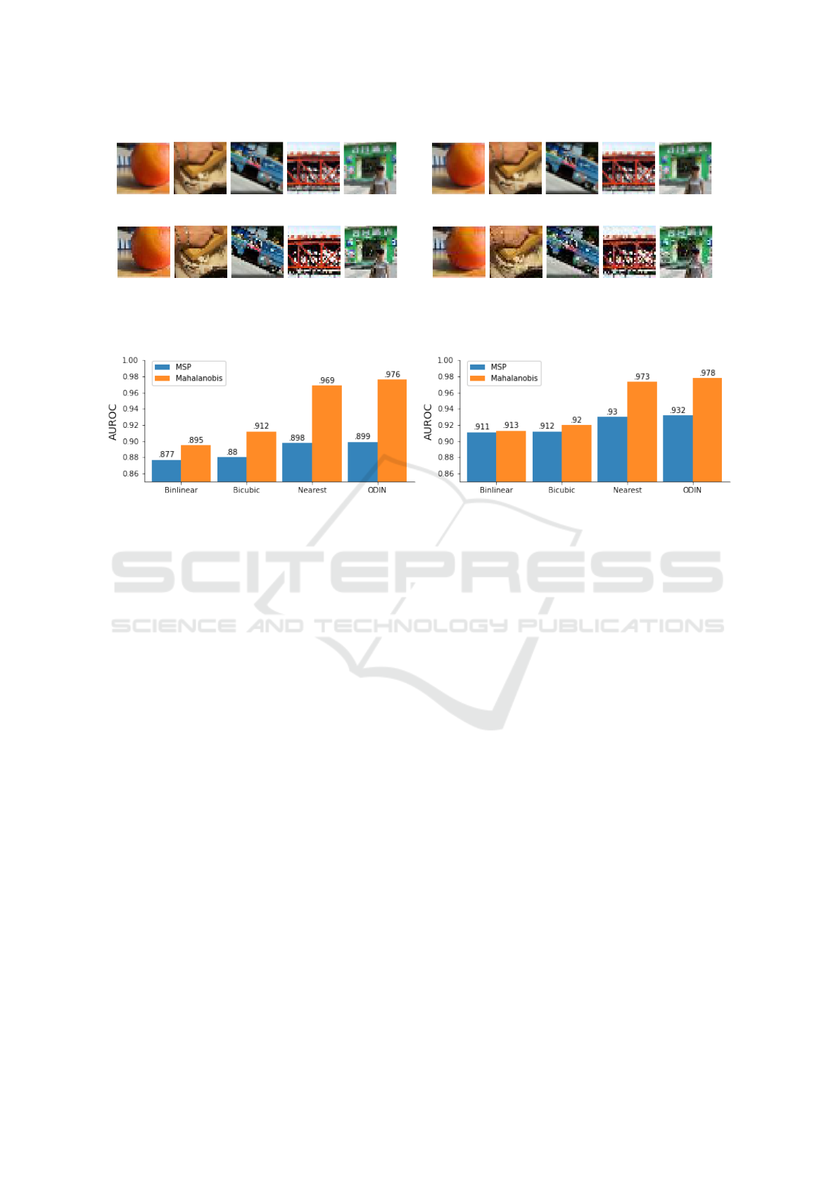
(a) Default PyTorch bilinear resize. (b) Pytorch bicubic resize.

Figure 1: Resized samples of the Tiny ImageNet dataset for different resizing methods. Different resizes produce different

images as noise can be introduced which can affect the OOD detection performance.

(a) Tiny ImageNet resizes. (b) LSUN resizes.

Figure 2: The AUROC scores for separating tiny ImageNet (2a) and LSUN (2b) with different resizes for both the baseline

model as well as the Mahalanobis distance based model. Different resizes lead to large differences in scores, indicating the

importance of the resize method and therefore the feature space.

CIFAR100 and Textures. This follows the stan-

dard OOD data setup followed by many such

as (Hendrycks and Gimpel, 2016; Lee et al., 2018;

Lee et al., 2017), but also the higher dimen-

sional OOD datasets used by (Huang and Li, 2021;

Hendrycks et al., 2019a; Roady et al., 2019). For a

correct OOD detection setting, we always use the ex-

act same test transform for the OOD data as for the

ID data. The resizing operation used for every OOD

dataset is the PyTorch default bilinear resizing opera-

tion.

Models. We ﬁrst train the RESNET34 model (He

et al., 2015) on the CIFAR10, CIFAR100 and SVHN

datasets from scratch, by using the training param-

eters provided by (Kuangliu, 2021) and obtain the

same performance. We then vary the training as de-

scribed in Section 3 and use the resulting model for

the MSP and Mahalanobis methods. The models are

then indicated as {model}-{variety} s.t. {model} ei-

ther indicates the MSP or Mahalanobis model, and

{variety} one of the training variations.

Metrics. The OOD detection on an ID-OOD dataset

pair can be viewed as a binary classiﬁcation problem,

where samples from the ID are labeled as positive

samples and samples from the OOD data as negative

samples. We then look at the Area Under the Re-

ceiver Operator Curve (AUROC), the Detection Ac-

curacy (Detection Acc.) and the True Negative Rate

at 95% True Positive Rate (TNR at TPR 95). These

are the generally included metrics for OOD detection.

Finally, in order to look at the relation between perfor-

mances, the Pearson correlation coefﬁcient is used.

4.2 Impact of Covariate Shift

This section describes two experiments that show how

the data is generally separated with an emphasis on

the covariate shift of the ID-OOD dataset pairs.

Resizing and Noise. For the preparation of ID-

OOD dataset pairs images might need to be resized.

For example, the images from CIFAR10 have a size of

32 × 32 while the images from Tiny ImageNet have a

size of 64×64 pixels. This means that in order to use

Tiny ImageNet as the OOD dataset, the images will

have to be resized to match the CIFAR10 data. Al-

though not a lot of attention has been brought to this

matter, from Figure 1 we can see that different resizes

produce different images. Especially in Figure 1c,

the resizing introduces a lot of noise into the images.

VISAPP 2023 - 18th International Conference on Computer Vision Theory and Applications

726

These images are very similar to the samples shown

in Figure 1d which come from the already resized

dataset that was open sourced by the authors of the

paper that introduced ODIN (Liang et al., 2017). Al-

though many have since used this data, to our knowl-

edge there has been no mention of the noise that is

present in the images and its effects.

In Figure 2, the Area Under the Receiver Oper-

ator Curve (AUROC) is plotted for the MSP model

and the Mahalanobis model for separating different

resizes of Tiny ImageNet and LSUN from CIFAR10.

The model has been trained using the default setup

explained in Section 3. We can see that especially

the Mahalanobis model performs a lot better depend-

ing on the resizing operation that is used, indicating

that it is detecting the noise in the images of the data

and using it to separate the OOD data from the ID

data. This makes sense, as the Mahalanobis distance

is the distance calculated in the feature space where

the noise in the images has a large impact. On the

other hand, the performance of the MSP model does

not increase as drastically for different resizing meth-

ods. This is likely because the class of the noisy im-

ages is still prominent despite the noise and that the

goal of the output layer is to ﬁnd that class, therefore

mainly ignoring the noise. To conclude, noise in the

OOD images can lead to an artiﬁcial increase in OOD

performance, especially for methods that utilize the

feature space. Since noise can be introduced because

of the resizing method, the resizing method must be

chosen carefully.

Covariate and Semantic Data Shift. Some sam-

ples from the OOD datasets can share classes with

the ID data. This can pose issues, as there is still

some controversy around if semantically similar sam-

ples should be viewed as OOD for the sake of gen-

eralization (Yang et al., 2021a; Yang et al., 2021b;

Huang and Li, 2021). For this reason, it is important

to investigate the relation between OOD performance

on samples that share a class and samples that do not

share a class with the ID data. This allows us to deter-

mine how the model separates the OOD from the ID

data and if it relies on semantics or not. More specif-

ically, we want to know if OOD detection methods

can actually make a distinction between the semantic

and covariate shift between the ID and OOD data. We

do so, by looking at the relation between the separa-

tion of semantically similar and semantically dissim-

ilar samples from the ID dataset.

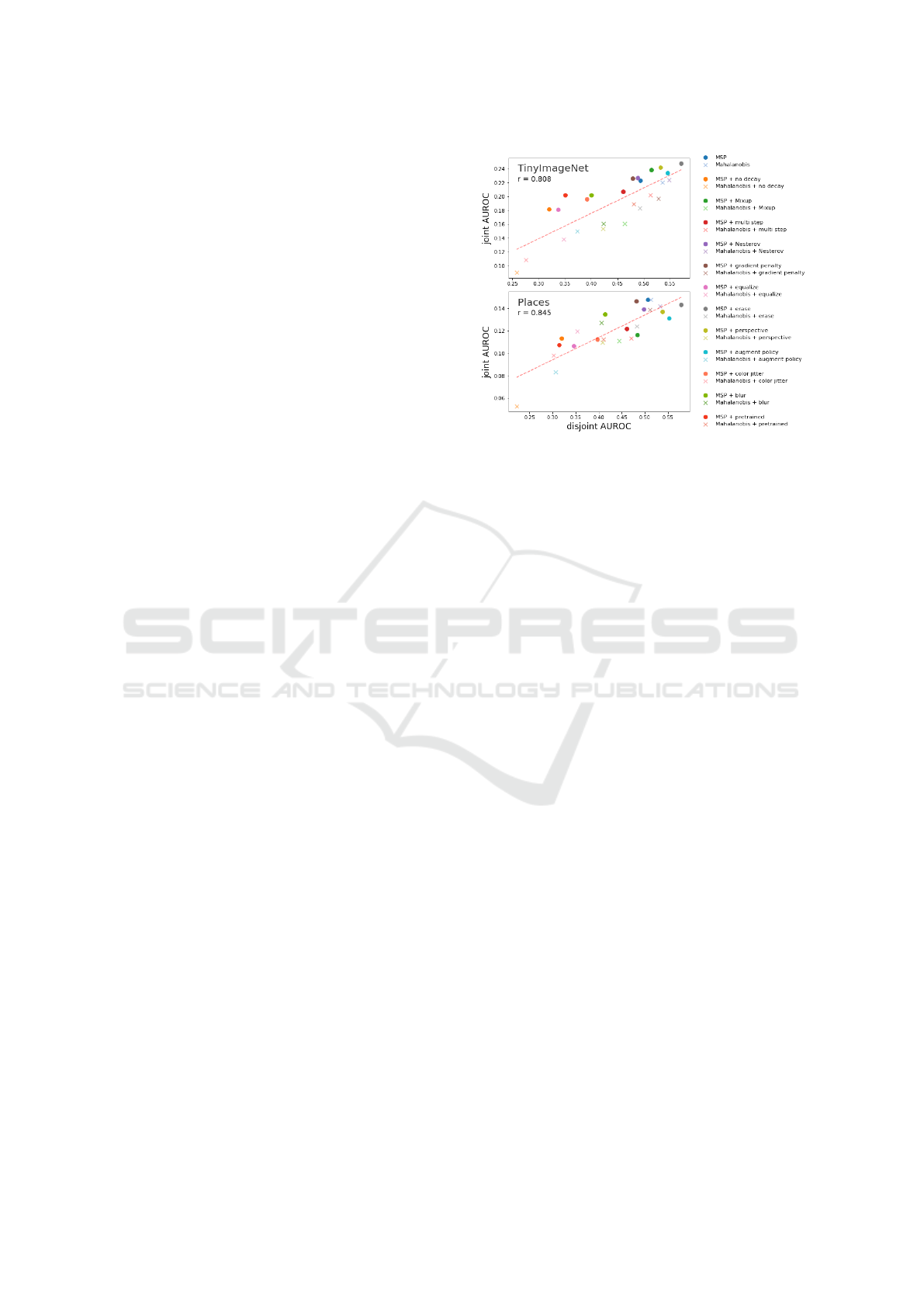
Figure 3 shows the AUROC for separating sam-

ples that do not share a class (disjoint), against the

AUROC for separating samples that do share a class

(joint) with the CIFAR10 dataset. In this ﬁgure, a

Figure 3: The AUROC for separating OOD samples that

share a class, against the AUROC for separating OOD sam-

ples that do not share a class with the CIFAR10 dataset.

The Tiny ImageNet and Places datasets are used as OOD

dataset. A fairly strong correlation between the two is visi-

ble.

fairly strong correlation between the two is shown.

This correlation indicates that if a model becomes bet-

ter at separating samples that share a class, it also be-

come better at separating samples that do not share a

class and vice versa.

Because samples with semantically dissimilar

classes can only be separated based on non-semantic

features, an increase in OOD performance can only

be explained by an increase in more discriminative

non-semantic features. Because there is a correla-

tion between the OOD performance for separating the

samples with disjoint classes and separating the sam-

ples with joint classes, it must be the case that the

samples with joint classes are also being separated

based on these non-semantic features. This means

that the methods at hand mostly separate the sam-

ples based on their covariate shift and not on their se-

mantic shift. However, it can be argued that semantic

features do not exist and that the semantic properties

of a model/image merely emerge from a set of non-

semantic features. Nevertheless, this would mean the

same thing, since the model would still be unable to

make a distinction between class dependent and in-

dependent features. From this, we can conclude that

the OOD detection depends on the covariate shift be-

tween the ID and OOD datasets.

However, as long as there are semantic differ-

ences, there must also be covariate differences. This

follows from the fact that a difference in class must

also lead to difference in images. If these differ-

ences are not captured by the model, it can be viewed

as a shortcoming of the model. Theoretically, as

The Effect of Covariate Shift and Network Training on Out-of-Distribution Detection

727

long as the feature space is descriptive and high-

level enough, separating any two semantically non-

overlapping datasets should be possible. The same

can however not be said for semantically overlapping

datasets, since semantically similar samples are not

bound to have different features given a more descrip-

tive feature space. This is only true if the features are

also on a high-enough level. For example, when two

sets of semantically non-overlapping images contain

the same low-level features, it becomes impossible to

separate them based on the low-level feature space.

4.3 CNN Training and OOD Detection

As the separation of ID and OOD data strongly de-

pends on the image features, looking at the effect of

the model training is important, because the model

training determines what features are learned. This

section provides insight about the effect of the train-

ing setup on the OOD detection performance.

CNN Accuracy and OOD Detection. When a

CNN is trained, the network learns different features

that aid to the minimization of the learning objec-

tive (Ilyas et al., 2019), and as we have shown in the

previous sections, the discriminativeness of the fea-

ture space is crucial for OOD detection. Therefore, by

training a model to have a more discriminative or less

discriminative feature space, the OOD detection per-

formance can be improved or diminished respectively.

This is in line with many other methods that use some

form of OOD data during training in order to obtain

more distinguishable features (Hendrycks et al., 2018;

DeVries and Taylor, 2018; Lee et al., 2017).

In order to investigate the effect of different train-

ing approaches on the OOD detection performance,

we trained several models on CIFAR10 with a single

difference in the setup in order to isolate its effect.

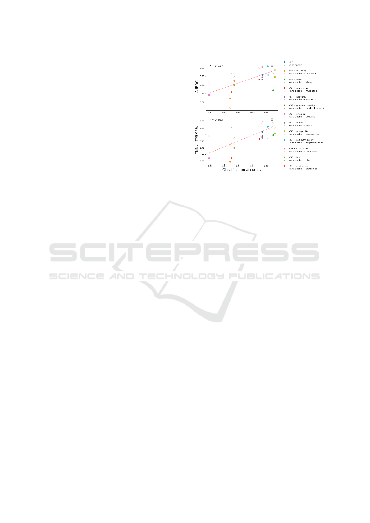
In Figure 4, we plotted the classiﬁcation accuracy of

the trained model, against the average AUROC and

average TNR at 95% TPR of the OOD performance

across all datasets for all of the training variations.

This ﬁgure shows a fairly strong correlation between

the classiﬁcation accuracy and the OOD performance,

although not very consistent.

For example, even though MixUp improves the

model accuracy, it reduces the OOD performance

with the MSP model compared to the basic MSP

model. Similarly, we see that when not using weight

decay or when using a multi step scheduler, that the

OOD performance is low compared to other training

variations with a similar accuracy. This shows that

although there is some correlation between the accu-

racy and OOD performance, that the individual train-

Figure 4: The accuracy against the average AUROC and

the average TNR at 95% TPR for all training variations. A

fairly strong correlation between the OOD performance and

the Accuracy is visible, but not very consistent.

ing methods have a bigger latent impact on the OOD

detection performance and are not necessarily related

to the accuracy of the model.

Benchmarking. By changing the training setup, the

classiﬁcation accuracy as well as the OOD detection

performance can be improved. Table 2 shows that

by changing the training approach, the OOD detec-

tion performance can be increased relative to the same

model with a different training setup. This table also

shows that when using the erase method, the perfor-

mance increases quite steadily with the exception of

the CIFAR100 dataset as ID dataset. Because ran-

dom patches are being set to random values, thereby

obscuring the images during training, the model is

forced to learn different and less typical features in

order to minimize the loss. Because these features are

more typical of the ID data and thus more distinguish-

able from the OOD data, they aid the OOD detection

performance.

When using the SVHN and Textures datasets as

OOD, the Mahalanobis method with erase consis-

tently performs the best. Conversely, when using the

SVHN dataset as the ID dataset, the Mahalanobis

method with erase performs the best for all OOD

datasets. This shows that the features learned by us-

ing the erase data augmentation are generally more

discriminative than without the erase data augmenta-

tion.

Although for the CIFAR10 and SVHN datasets

the erase method performs the best, both with the

MSP or the Mahalanobis model, the CIFAR100

dataset deviates from this trend. From the table it

VISAPP 2023 - 18th International Conference on Computer Vision Theory and Applications

728

Table 2: The OOD detection results for the commonly used ID-OOD dataset pairs and several metrics. The MSP and

Mahalanobis distance on the default setup as well as the MSP and Mahalanobis distance with the erase data augmentation

setup variations are shown. The highest scores are printed in bold.

MSP / Mahalanobis / MSP + erase / Mahalanobis + erase

ID OOD AUROC Detection acc. TNR at TPR 95%

CIFAR10 SVHN .947 / .966 / .971 / .987 .920 / .941 / .950 / .958 .662 / .786 / .830 / .938

TinyImageNet .877 / .895 / .897 / .891 .827 / .829 / .845 / .824 .461 / .498 / .533 / .456

LSUN .911 / .913 / .930 / .911 .857 / .850 / .878 / .848 .511 / .514 / .595 / .475

Places .893 / .899 / .912 / .899 .872 / .878 / .889 / .884 .494 / .500 / .563 / .470

CIFAR100 .881 / .896 / .905 / .895 .827 / .830 / .852 / .826 .446 / .492 / .525 / .457

Textures .914 / .968 / .928 / .983 .855 / .905 / .873 / .933 .544 / .799 / .594 / .903

CIFAR100 SVHN .723 / .840 / .785 / .894 .777 / .817 / .811 / .869 .142 / .363 / .197 / .412

TinyImageNet .801 / .806 / .790 / .737 .737 / .745 / .728 / .687 .246 / .236 / .227 / .119

LSUN .749 / .726 / .748 / .645 .700 / .685 / .697 / .624 .152 / .122 / .141 / .054

Places .775 / .766 / .773 / .699 .818 / .805 / .826 / .802 .207 / .201 / .195 / .094

CIFAR10 .783 / .753 / .775 / .628 .719 / .708 / .713 / .612 .216 / .157 / .197 / .042

Textures .787 / .931 / .805 / .951 .718 / .852 / .727 / .882 .204 / .658 / .248 / .745

SVHN CIFAR10 .913 / .983 / .930 / .994 .893 / .942 / .891 / .967 .715 / .922 / .721 / .982

TinyImageNet .915 / .984 / .923 / .995 .895 / .944 / .889 / .970 .725 / .927 / .714 / .983

LSUN .899 / .981 / .906 / .994 .885 / .939 / .879 / .968 .680 / .906 / .674 / .985

Places .909 / .984 / .920 / .995 .869 / .950 / .867 / .973 .704 / .921 / .703 / .988

CIFAR100 .913 / .983 / .923 / .993 .892 / .941 / .888 / .965 .713 / .917 / .711 / .980

Textures .893 / .991 / .890 / .997 .904 / .963 / .898 / .980 .684 / .963 / .651 / .991

is evident that with the exception of the SVHN and

Textures datasets, the standard MSP and Mahalanobis

models perform the best when using CIFAR100 as ID

data. This is likely the case because when training on

the CIFAR100 data, the model learns more different

features than when training on CIFAR10 or SVHN.

This means that the features from the OOD datasets

are more likely to be present in the known features of

the model due to its inclusiveness. This also explains

why Mixup obtains high accuracy but a low OOD per-

formance. Due to the more inclusive features, the fea-

tures of the OOD data are more likely to fall within

the same range as the features of the ID data.

5 CONCLUSION

We have shown that current OOD detection meth-

ods rely heavily on the difference in features between

datasets and are therefore only able to detect the co-

variate shift. This reliance on covariate shift poses

some future problems since detecting the semantic

shift between images is debatably just as crucial.

The model training can then be altered in order

to obtain better OOD detection methods. In this

work we have highlighted the erase data augmenta-

tion, which obtains the best performance with only

a single adaption to the training procedure for most

ID-OOD dataset pairs. When using the erase method

in combination with the Mahalanobis distance, it also

consistently obtains the best results when using the

SVHN and Textures datasets as OOD.

Although model training seems to be a useful tool

for improving OOD detection performance, it does

come with problems. As seen in Table 2, when us-

ing CIFAR100 as ID dataset, the OOD performance

drops as opposed to the other ID datasets. This likely

happens because of the more inclusive feature space

learned by the model. A similar phenomenon is also

seen when using Mixup to train the CNN, although

the accuracy improves, the OOD performance is rel-

atively low. This also makes it difﬁcult to state that

a richer feature space would lead to better OOD per-

formance, as it can go both ways. It is therefore more

fair to state that a more discriminative feature space

leads to better OOD performance and that a more dis-

criminative feature space is often the result of a richer

feature space.

As a future work, it should be investigated what

it means to have a more discriminative feature space

as opposed to a rich feature space. When does a

model become more inclusive and when does it be-

come more discriminative? Conversely, how can we

deﬁne discriminative and inclusiveness in OOD de-

tection? These research questions pair well with the

investigation of Mixup, which obtains better classiﬁ-

cation performance but does not increase OOD detec-

tion performance, as well as the investigation of why

the OOD performance when training on CIFAR100 is

so different from the OOD performance when training

The Effect of Covariate Shift and Network Training on Out-of-Distribution Detection

729

on CIFAR10. We believe that these future research

questions combined with the results from this paper

pave the way for safer use of neural networks.

REFERENCES

Betta, G., Capriglione, D., Liguori, C., and Paolillo, A.

(2011). Uncertainty Evaluation in Face Recognition

Algorithms. IEEE International Instrumentation and

Measurement Technology Conference (I2MTC).

Boone, L., Biparva, M., Forooshani, P. M., Ramirez, J.,

Masellis, M., Bartha, R., Symons, S., Strother, S.,

Black, S. E., Heyn, C., Martel, A. L., Swartz, R. H.,

and Goubran, M. (2022). ROOD-MRI: Benchmarking

the Robustness of Deep Learning Segmentation Mod-

els to Out-of-Distribution and Corrupted Data in MRI.

Technical report.

Chang, J., Lan, Z., Cheng, C., and Wei, Y. (2020). Data

Uncertainty Learning in Face Recognition. In CVPR.

Corbi

ere, C., Thome, N., Bar-Hen, A., Cord, M., and P

erez,

P. (2019). Addressing Failure Prediction By Learning

Model Conﬁdence. In NeurIPS.

Cubuk, E. D., Zoph, B., Mane, D., Vasudevan, V., and Le,

Q. V. (2019). Autoaugment: Learning augmentation

strategies from data. In CVPR.

DeVries, T. and Taylor, G. W. (2018). Learning Conﬁdence

for Out-of-Distribution Detection in Neural Networks.

Technical report.

Drucker, H. and Cun, Y. L. (1992). Improving General-

ization Performance Using Double Backpropagation.

IEEE Transactions on Neural Networks.

Fort, S., Ren, J., and Lakshminarayanan, B. (2021). Ex-

ploring the Limits of Out-of-Distribution Detection.

In NeurIPS.

He, K., Zhang, X., Ren, S., and Sun, J. (2015). Deep Resid-

ual Learning for Image Recognition. Technical report.

Hendrycks, D., Basart, S., Mazeika, M., Zou, A., Kwon, J.,

Mostajabi, M., Steinhardt, J., and Song, D. (2019a).

A Benchmark for Anomaly Segmentation.

Hendrycks, D., Basart, S., Mazeika, M., Zou, A., Kwon, J.,

Mostajabi, M., Steinhardt, J., and Song, D. (2019b).

Scaling Out-of-Distribution Detection for Real-World

Settings. In ICML.

Hendrycks, D. and Gimpel, K. (2016). A Baseline for De-

tecting Misclassiﬁed and Out-of-Distribution Exam-

ples in Neural Networks. In ICLR.

Hendrycks, D., Mazeika, M., and Dietterich, T. (2018).

Deep Anomaly Detection with Outlier Exposure. In

ICLR.

Huang, R. and Li, Y. (2021). MOS: Towards Scaling Out-

of-distribution Detection for Large Semantic Space.

In CVPR.

Ilyas, A., Santurkar, S., Tsipras, D., Engstrom, L., Tran, B.,

and Madry, A. (2019). Adversarial Examples Are Not

Bugs, They Are Features. In NeurIPS.

Kuangliu (2021). Kuangliu/Pytorch-CIFAR: 95.47% on CI-

FAR10 with pytorch.

Lee, K., Lee, H., Lee, K., and Shin, J. (2017). Training

Conﬁdence-calibrated Classiﬁers for Detecting Out-

of-Distribution Samples. In ICLR.

Lee, K., Lee, K., Lee, H., and Shin, J. (2018). A Simple

Uniﬁed Framework for Detecting Out-of-Distribution

Samples and Adversarial Attacks. NeurIPS.

Liang, S., Li, Y., and Srikant, R. (2017). Enhancing the

Reliability of Out-of-Distribution Image Detection in

Neural Networks. ICLR.

Liu, W., Wang, X., Owens, J. D., and Li, Y. (2020). Energy-

based Out-of-distribution Detection. In NeurIPS.

Mehrtash, A., Wells, W. M., Tempany, C. M., Abolmae-

sumi, P., and Kapur, T. (2020). Conﬁdence Calibra-

tion and Predictive Uncertainty Estimation for Deep

Medical Image Segmentation. IEEE Transactions on

Medical Imaging.

Nesterov, Y. E. (1983). A Method of Solving a Convex

Programming Problem With Convergence rate. Pro-

ceedings of the USSR Academy of Sciences.

Raghu, M., Blumer, K., Sayres, R., Obermeyer, Z., Klein-

berg, R., Mullainathan, S., and Kleinberg, J. (2019).

Direct Uncertainty Prediction for Medical Second

Opinions. In ICML.

Roady, R., Hayes, T. L., Kemker, R., Gonzales, A., and

Kanan, C. (2019). Are Out-of-Distribution Detection

Methods Effective on Large-Scale Datasets? Techni-

cal report.

Sastry, C. S. and Oore, S. (2020). Detecting Out-of-

Distribution Examples with Gram Matrices. In ICML.

Sun, Y., Guo, C., and Li, Y. (2021). ReAct: Out-of-

distribution Detection With Rectiﬁed Activations. In

NeurIPS.

Vojir, T., Sipka, T., Aljundi, R., Chumerin, N., Olmeda

Reino, D., and Matas, J. (2021). Road Anomaly De-

tection by Partial Image Reconstruction with Segmen-

tation Coupling. In ICCV.

Winkens, J., Bunel, R., Roy, A. G., Stanforth, R., Natara-

jan, V., Ledsam, J. R., MacWilliams, P., Kohli, P.,

Karthikesalingam, A., Kohl, S., Cemgil, T., Eslami,

S. M. A., and Ronneberger, O. (2020). Contrastive

Training for Improved Out-of-Distribution Detection.

Technical report.

Yang, J., Wang, H., Feng, L., Yan, X., Zheng, H.,

Zhang, W., and Liu, Z. (2021a). Generalized Out-of-

Distribution Detection: A Survey. Technical report.

Yang, J., Wang, H., Feng, L., Yan, X., Zheng, H., Zhang,

W., and Liu, Z. (2021b). Semantically Coherent Out-

of-Distribution Detection. In ICCV.

Zhang, H., Cisse, M., Dauphin, Y. N., and Lopez-Paz, D.

(2018). MixUp: Beyond Empirical Risk Minimiza-

tion. In ICLR.

Zhong, Z., Zheng, L., Kang, G., Li, S., and Yang, Y. (2020).

Random Erasing Data augmentation. In Proceedings

of the AAAI Conference on Artiﬁcial Intelligence.

Zisselman, E. and Tamar, A. (2020). Deep Residual Flow

for Out of Distribution Detection. In CVPR.

VISAPP 2023 - 18th International Conference on Computer Vision Theory and Applications

730