Shufﬂe Mixing: An Efﬁcient Alternative to Self Attention

Ryouichi Furukawa

and Kazuhiro Hotta

Meijo University, 1-501 Shiogamaguchi, Tempaku-ku, Nagoya 468-8502, Japan

Keywords:

Transformer, Self Attention, Depth Wise Convolution, Shift Operation.

Abstract:

In this paper, we propose ShufﬂeFormer, which replaces Transformer’s Self Attention with the proposed shuf-

ﬂe mixing. ShufﬂeFormer can be ﬂexibly incorporated as the backbone of conventional visual recognition,

precise prediction, etc. Self Attention can learn globally and dynamically, while shufﬂe mixing employs Depth

Wise Convolution to learn locally and statically. Depth Wise Convolution does not consider the relationship

between channels because convolution is applied to each channel individually. Therefore, shufﬂe mixing can

obtain the information on different channels without changing the computational cost by inserting a shift op-

eration in the spatial direction of the channel direction components. However, by using the shift operation, the

amount of spatial components obtained is less than that of Depth Wise Convolution. ShufﬂeFormer uses over-

lapped patch embedding with a kernel larger than the stride width to reduce the resolution, thereby eliminating

the disadvantages of using the shift operation by extracting more features in the spatial direction. We evaluated

ShufﬂeFormer on ImageNet-1K image classiﬁcation and ADE20K semantic segmentation. ShufﬂeFormer has

superior results compared to Swin Transformer. In particular, ShufﬂeFormer-Base/Light outperforms Swin-

Base in accuracy at about two-thirds of the computational cost.

1 INTRODUCTION

In computer vision, network design plays an impor-

tant role in improving performance. The recently de-

veloped Vision Transformer(ViT) (Sharir et al., 2021)

has the potential to surpass convolution, which has

dominated the ﬁeld since the AlexNet (Krizhevsky

et al., 2017). The superiority of ViT was ﬁrst

demonstrated in image classiﬁcation tasks, and ViT

is rapidly spreading to many other tasks such as

semantic segmentation (Strudel et al., 2021), ob-

ject detection (Chi et al., 2020), and action recog-

nition (Arnab et al., 2021). ViT consists of Posi-

tional Embedding and multiple Transformer Encoders

which are composed of Normalization, Self Attention

(Vaswani et al., 2017), and FFN. The superiority of

ViT over convolution has been attributed to Self At-

tention which can model spatial relationships dynami-

cally and globally. Speciﬁcally, Self Attention extract

features from arbitrary locations using weights calcu-

lated by using inner products. Self Attention has two

advantages compared to convolution. First, the en-

tire image is treated as input, so local constraints in

convolution can be ignored. Second, the weights are

dynamically generated by input features, rather than

ﬁxed weights generated by training as in convolution.

https://orcid.org/0000-0002-8723-7742

https://orcid.org/0000-0002-5675-8713

However, can the advantages be considered a fac-

tor in ViT’s success? Local attention mechanism is

introduced to ViTs to restrict their attention scope

within a small local region, e.g., Swin Transformer

(Liu et al., 2021b) and Local ViT (Li et al., 2021). The

results indicate that local restrictions do not degrade

performance. MLP-Mixer (Tolstikhin et al., 2021)

substitutes Self Attention for a linear projection layer

used in spatial direction and achieves top performance

on ImageNet-1K (Russakovsky et al., 2015). More

surprisingly, MetaFormer (Yu et al., 2022), which re-

placed Self Attention with a simple pooling mech-

anism, also performed very well. These results in-

dicate that dynamic weight generation is not neces-

sarily important. Therefore, the success of ViT may

not be due to Self Attention, which was previously

considered to be important, but to the other network

structures and learning methods. In addition, Self At-

tention has the following problems, which have been

discussed in many conventional types of pieces of

research (Katharopoulos et al., 2020). The compu-

tational cost of Self Attention is proportional to the

square of the number of patches in the input image.

This causes signiﬁcant computational cost problems

for most tasks in computer vision that deal with two-

dimensional information.

We considered that an important approach to cre-

ate a superior model to ViT from these perspectives

700

Furukawa, R. and Hotta, K.

Shufﬂe Mixing: An Efﬁcient Alternative to Self Attention.

DOI: 10.5220/0011720200003417

In Proceedings of the 18th International Joint Conference on Computer Vision, Imaging and Computer Graphics Theory and Applications (VISIGRAPP 2023) - Volume 5: VISAPP, pages

700-707

ISBN: 978-989-758-634-7; ISSN: 2184-4321

 2023 by SCITEPRESS – Science and Technology Publications, Lda. Under CC license (CC BY-NC-ND 4.0)

would be to replace self-attention with methods that

are computationally less expensive and to improve

methods such as FFN, Patch Embedding, and Nor-

malization. In this paper, we focus on Depth Wise

convolution (DWconv) (Howard et al., 2017) and shift

operations (Wang et al., 2022) to create a more ef-

ﬁcient (low computational cost and high accuracy)

method than Self Attention. The block of our pro-

posed method consists of Token Mixer for spatial

modeling and FFN for channel modeling, similar to

the Transformer structure handled in computer vi-

sion. In the proposed method, Token Mixer is re-

placed with the proposed shufﬂe mixing, and FFN is

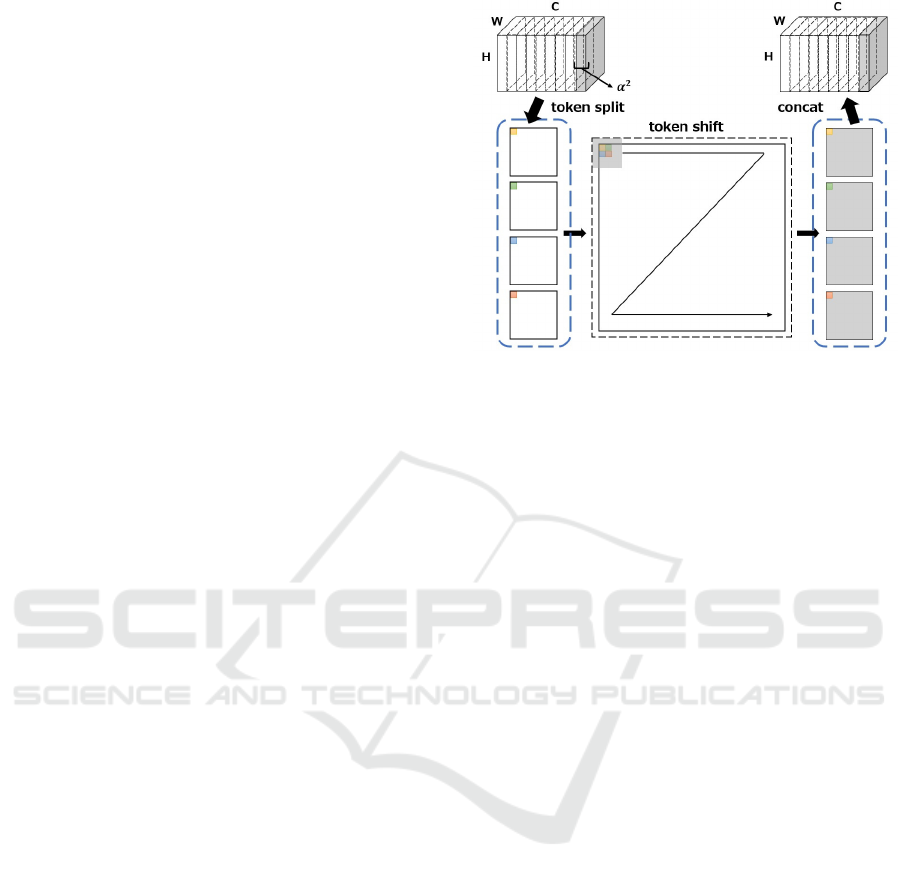
retained. First, the proposed shufﬂe mixing as shown

in Figure 1 shifts the features in the channel direc-

tion to neighboring spatial neighborhoods on the same

coordinates. Next, DWconv with an increased num-

ber of output channels can be used to extract nearby

channels and spatial direction components without in-

creasing computational cost. Shufﬂe mixing limits

the ability to model in the spatial direction by using

shift to allow reference to components in the channel

direction. Therefore, the ability to acquire spatial in-

formation is compensated for by increasing the size of

the kernel of patch embedding, which performs reso-

lution reduction.

The proposed ShufﬂeFormer using these blocks

and patch embedding achieved the same or better ac-

curacy than Swin Transformer. Speciﬁcally, on the

ImageNet-1k dataset with the same computational

complexity as Swin-B, our ShufﬂeFormer achieved

an accuracy improvement of 0.62%. Furthermore, in

comparison with Swin-B/Light, our model achieved

the same accuracy while reducing the computational

cost by two-thirds. Our method also achieved a 0.5%

mIoU improvement in semantic segmentation on the

ADE20K dataset (Zhou et al., 2019), which has the

same computational complexity as Swin-B.

This paper is organized as follows. Section 2 de-

scribes the related works. The detail of the proposed

method is presented in section 3. Section 4 shows the

experimental results. Finally, section 5 provides con-

clusions and future work.

2 RELATED WORKS

Transformer (Vaswani et al., 2017) is a model de-

veloped in natural language processing(NLP). RNN

(Mikolov et al., 2010) conventionally used in NLP

has the problem of not being able to parallelize the

computation because the hidden state obtained from

the previous time is used as input for processing at

the next time. CNN does not need to input the infor-

Figure 1: Overview of shufﬂe mixing.

mation obtained from the previous time as RNN, so

the computation can be parallelized. However, CNN

(LeCun et al., 1989) has the problem that it is difﬁ-

cult to capture distant information. Transformer has

achieved great success in NLP because it can paral-

lelize computations unlike existing RNNs and CNNs

while capturing the relationship between distant in-

formation.

ViT (Sharir et al., 2021) is a typical model that uti-

lizes the Transformer for computer vision. ViT solved

the local constraints of CNNs, which have been a

problem in computer vision as well, by dividing the

image into patches and inputting them to the Trans-

former. In addition, ViT allows the weights to be han-

dled dynamically. Following the success of ViT, many

studies using Transformer have been conducted in

computer vision. CoAtNet (Dai et al., 2021) and CmT

(Guo et al., 2022) improve the performance by mixing

convolution and Self Attention, while CvT (Wu et al.,

2021) improves the performance by introducing con-

volution in the Self Attention embedding layer. PVT

(Wang et al., 2021) includes downsampling in ViT,

making it easier to apply ViT to other tasks except

for image classiﬁcation. There is no improvement in

Transformer’s Self Attention in these methods, which

still guarantees the success of the vanilla Transformer

in computer vision.

However, is it really possible to say that Self At-

tention has led to Transformer’s success? Self Atten-

tion has the disadvantage that the computational cost

is the square of the size of the input token. Swin

Transformer achieved better performance than ViT

while reducing computational cost by restricting im-

ages to local regions called windows and inputting

each window to Self Attention. MLP-Mixer (Tol-

stikhin et al., 2021) used token-mixing MLP, which

learns all spatial information by linear projection

Shufﬂe Mixing: An Efﬁcient Alternative to Self Attention

701

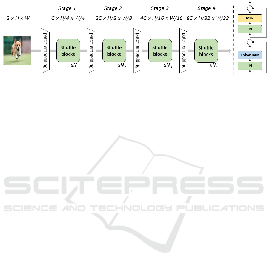
Figure 2: Left: Overview of Shufﬂeformer, Right: Overview of shufﬂe block

layer, instead of Self Attention. However, it lacks the

property of dynamically handling weights. In subse-

quent studies, spatial gating units (Liu et al., 2021a)

and cyclic connections (Chen et al., 2021) have been

used similarly with high success using MLP in the

spatial direction. These studies suggest that the global

feature extraction and dynamic weighting properties

of Self Attention do not necessarily lead to the suc-

cess of Transformer in computer vision. The fact that

PoolFormer (Yu et al., 2022), which replaces Self At-

tention with a simple average pooling layer, works as

well as the latest Networks, increases the possibility

that the consideration is correct.

In these research trends, our model is similar to

PoolFormer in that it replaces Self Attention with a

method that has local and static weights. To create

an efﬁcient model, Self Attention is replaced by a

method using DWconv and shift operations. The pro-

posed method can extract features by DWconv more

effectively than average pooling, and refer to infor-

mation from different channels by using shift with-

out changing the computational cost. We demonstrate

the usefulness of the proposed method by comparing

the Self Attention-based method and vanilla DWconv

through experiments.

3 PROPOSED METHOD

3.1 Network Architecture

For comparison with networks using Self Attention,

ShufﬂeFormer takes on the structure shown in Figure

2. For hierarchical feature extraction such as PVT,

overlapped patch embedding is used for resolution re-

duction. Patch embedding used in Swin Transformer

is implemented using convolution with equal kernel

size and stride. In overlapped patch embedding, the

kernel size is made larger than the stride width to gen-

erate patches with more spatial information. Shufﬂe-

Former consists of four stages. The i-th stage consists

of an overlapped patch embedding layer and multi-

ple shufﬂe blocks. In actuality, we use a convolution

layer with a kernel size of 7 × 7 and stride of 4 ×

4, and output as an arbitrary number of channels C

(output features are H/4 × W/4 × C). Unlike con-

ventional methods, this method takes duplicates into

account, and thus generates better patches for a larger

computational cost.

Next, the generated patches are used as input to

the shufﬂe block for feature extraction. The same

structure is used in stages 2, 3, and 4 for feature ex-

traction. The number of channels is doubled by using

a convolution layer with a kernel size of 3 × 3 and

a stride of 2 for the Patch embedding layer of each

stage. That is, the output resolutions of stages 2, 3,

and 4 are H/8 × W /8,H/16 × H/16, and H/32 ×

W /32, and the corresponding channel numbers are

2C, 4C, and 8C, respectively. Since the network

outputs features of different resolutions at different

stages, it can be used for tasks such as segmenta-

tion and object detection as well as conventional CNN

methods.

3.2 Shufﬂe Block

3.2.1 Composition of Block

The shufﬂe block takes features from the patch em-

bedding layer as input. As shown in Figure 2, the

shufﬂe block consists of shufﬂe mixing, FFN, nor-

malization, and residual connection. FFN consists of

two linear transformation layers and a GELU func-

tion. Layer Norm (LN) is used for Normalization.

Therefore, a shufﬂe block is deﬁned as follows.

′

= x + shufﬂemixing(LN(x))

y = x

′

+ FFN(LN(x

′

))

where x ∈ R

h×w×c

, h, w is the height and width of in-

put feature, and c is the number of dimensions.

VISAPP 2023 - 18th International Conference on Computer Vision Theory and Applications

702

Table 1: Model Conﬁguration. Block Num indicates the number of blocks in each Stage of Shufﬂeformer. Embedded

Dimension indicates the number of channels in each Stage. /Light model has the same conﬁguration as the Swin Transformer

model being compared, while the model without /Light has a modiﬁed Block Num conﬁguration to keep Pram and FLOP

comparable to the Swin Transformer.

Model Size Block Num Embedded Dimension MLP Ratio Param(M) FLOPs(G)

Minute {2, 2, 6, 2} {64, 128, 320, 512} {4, 4, 4, 4} 12.0 1.85

Tiny/Light {2, 2, 6, 2} {96, 192, 382, 764} {4, 4, 4, 4} 21.7 3.26

Tiny {3, 4, 8, 3} {96, 192, 382, 764} {4, 4, 4, 4} 29.5 4.67

Small/Light {2, 2, 18, 2} {96, 192, 382, 764} {4, 4, 4, 4} 36.0 6.06

Small {4, 8, 20, 4} {96, 192, 382, 764} {4, 4, 4, 4} 49.8 8.9

Base/Light {2, 2, 18, 2} {128, 256, 512, 1024} {4, 4, 4, 4} 63.5 10.7

Base {4, 8, 20, 4} {128, 256, 512, 1024} {4, 4, 4, 4} 88.0 15.7

3.2.2 Shufﬂe Mixing

Shufﬂe mixing is the replacement of Self Attention

in Transformer, and shufﬂe mixing should be a low-

cost feature extractor which is the purpose of this pa-

per. Shufﬂe mixing consists of shift operation and

DWconv. DWconv is known as a very lightweight

feature extraction method because one channel corre-

sponds to one ﬁlter. However, DWconv makes it im-

possible to refer the features between different chan-

nels. Grouped Convolution can refer different chan-

nels, but the parameters and FLOPs increase by the

number of groups. Shufﬂe mixing enables to refer

the features in different channels without increasing

parameters or FLOPs by performing DWconv after

shifting features in the channel direction in the spa-

tial direction. Speciﬁcally, as shown in Figure 1, the

feature map is segmented by a constant Group α

and

then the pixels of each channel are shifted to the same

coordinates. Therefore, the generated features have

different channels in the spatial direction, but the res-

olution is multiplied by α. Perform the DWconv with

kernel size k × k and stride α × α on the feature af-

ter shift operation. To make the ﬁnal output equal to

the input features, DWconv outputs α × α channels

per channel. However, shufﬂe mixing has a smaller

reference range in the spatial direction than regular

DWConv. Therefore, the overlapped patch embed-

ding shown in section 3.1 is supplemented with refer-

ences in the spatial direction by using a kernel larger

than the conventional method. The larger the value

of α, the larger the kernel size should be so that both

the channel and spatial direction components can be

referenced after shifting. In this paper, the value of

α was set to 2 and a kernel size k of 5 was used to

reduce computational cost.

3.3 Model Conﬁguration

To make a fair comparison with conventional meth-

ods, we constructed several models with a different

number of parameters and computational complexity

as shown in Table 1. Speciﬁcally, among the mod-

els, Shufﬂe-M(inute) corresponds to MetaFormer-

S12 (Yu et al., 2022). The other models Shufﬂe-

T(iny), S(mall), and B(ase) correspond to Swin-T, S,

and B (Liu et al., 2021b), respectively.

Models with /Light have the same number of lay-

ers and channels as Swin, and models without /Light

have the same parameters and FLOPs as Swin, but

with more layers. For the models handled in this

paper, the MLP channel expansion ratio is set to

4. Additionally, we set the stochastic depth (Huang

et al., 2016) rate as 0.1/0.1/0.3/0.4 respectively for our

ShufﬂeFormer-M/T/S/B.

4 EXPERIMENTS

We conduct experiments on ImageNet-1K (Rus-

sakovsky et al., 2015) image classiﬁcation and

ADE20K (Zhou et al., 2019) semantic segmenta-

tion. In the following, we ﬁrst compare the pro-

posed Shufﬂeformer architecture with the conven-

tional method. Then, an ablation study was performed

with ImageNet-1K.

4.1 Classiﬁcation on ImageNet-1K

4.1.1 Experimental Setting

We evaluated the performance of ShufﬂeFormer on

ImageNet-1K, which consists of 1.28M training im-

ages with 1000 classes and 50K validation images.

To validate the effectiveness of ShufﬂeFormer and to

fairly compare it with conventional methods, the fol-

lowing settings were used. We experimented with two

nvidia A6000 GPUs. The batch size per GPU was set

to 128 for all methods, and we trained all methods for

300 Epochs. The optimization method was AdamW

(Loshchilov and Hutter, 2017) with a weight decay

of 0.05 and a momentum of 0.9. The cosine decay

Shufﬂe Mixing: An Efﬁcient Alternative to Self Attention

703

Table 2: Experimental results on ImageNet-1K and ADE20K datassets. In experiments on ImageNet-1K, our method is

compared to ResNet (He et al., 2016), RegNet (Radosavovic et al., 2020), and Swin Transformer. For ADE20K, we used

Semantic FPN (Kirillov et al., 2019) with pre-trained model on ImageNet-1K as the backbone.

ImageNet-1K ADE20k

Model Param(M) FLOPs(G) Top-1 Semantic FPN

Acc.(%) mIoU(%)

ResNet-50 26 4.1 76.93 36.5

RegNet-4G 21 4.0 79.82 39.6

Swin-T 29 4.5 80.91 40.6

Shufﬂe-T/L 22 3.3 79.94 39.7

Shufﬂe-T 30 4.7 81.41 40.9

RegNet-8G 39 8.0 81.49 40.9

Swin-S 50 8.7 81.99 42.9

Shufﬂe-S/L 36 6.1 81.98 42.6

Shufﬂe-S 50 8.9 82.44 43.3

RegNet-16G 84 16.0 82.03 42.7

Swin-B 88 15.4 82.20 43.2

Shufﬂe-B/L 64 10.7 82.24 43.5

Shufﬂe-B 88 15.7 82.82 43.8

learning rate scheduler (Loshchilov and Hutter, 2016)

and 5 epochs of a linear warm-up are used. The ini-

tial learning rate was 1e

−6

, warming up to 3.75e

−4

and ﬁnally down to 1e

−5

. Data Augmentation was

applied using Rang Augment (Cubuk et al., 2020),

Mixup (Zhang et al., 2017), Cutmix (Yun et al., 2019),

CutOut (Zhong et al., 2020), and all parameters were

set the same as in the DeiT (Touvron et al., 2021) ex-

periment.

4.1.2 Results

Table 2 compares the classiﬁcation accuracy, compu-

tational cost (FLOPs), and parameters for each net-

work on the ImageNet-1K validation images. The

best accuracy is written in red ink in the table. Com-

paring the accuracy of Shufﬂeformer-{T, S, B} with

conventional methods with similar computational pa-

rameters and costs, the proposed method outper-

forms them for all model sizes. In addition, the

shufﬂeformer-{S/Light, B/Light} achieved the same

accuracy despite lower parameters and cost than Swin

Transformer. From this result, it can be considered

that the combination of patch embedding, which in-

creases the kernel size of ShufﬂeFormer, and shufﬂe

mixing, which can efﬁciently extract different channel

components, is effective for efﬁcient model construc-

tion.

4.2 Semantic Segmentation on ADE20K

4.2.1 Experimental Setting

To show the effectiveness of our method for seman-

tic segmentation, we evaluated our method on the

ADE20k dataset which consists of 20K training im-

ages with 150 classes and 2K validation images Our

codes are based on mmseg. We adopt the popular Se-

mantic FPN as the basic framework. For a fair com-

parison, we evaluated with Semantic FPN (Kirillov

et al., 2019) using cosine scheduling with 80k itera-

tions, similar to the PVT (Wang et al., 2021) setting.

4.2.2 Results

Table 2 shows the results of various models

pre-trained on ImageNet-1K as the backbone.

ShufﬂeFormer-{T,S, B} successfully improved the

accuracy by {0.3,0.4, 0.6%} to Swin-{T, S, B}.

The results show that our method outperforms the

Swin Transformer in the segmentation task. In

the lightweight model (/Light), our method outper-

formed Swin-B by 0.3% in the case of ShufﬂeFormer-

B/Light, which has a larger model size. These results

demonstrated that our model is more efﬁcient than the

Swin Transformer.

4.3 Ablation Study on ImageNet-1K

4.3.1 Comparison of Token Mixing

To verify the effectiveness of shufﬂe mixing, we will

compare the accuracy when Token Mixing is replaced

VISAPP 2023 - 18th International Conference on Computer Vision Theory and Applications

704

with a method that has the nearly same FLOPs. Ac-

curacy comparison of shufﬂe mixing in the proposed

ShufﬂeformerM, T/Light with average pooling (Yu

et al., 2022), shift operation (Wang et al., 2022), and

DWconv. Since the kernel size used for shufﬂe mix-

ing in this paper is 5, the kernel sizes of average pool-

ing and DWconv used in this experiment are set to 5.

Table 3 compares the classiﬁcation accuracy,

FLOPs, and parameters of each network when we

evaluated on ImageNet validation. The best accu-

racy is written in red ink in the table.. When we

compare the proposed method with 0 FLOPs, 0-

parameter average pooling, and shift operation. The

increase in computational parameters and FLOPs is

also minimal. These results conﬁrm that shufﬂe mix-

ing is a very computationally inexpensive method.

In terms of accuracy, Shufﬂe-M improves by 1.06%

from average pooling and 0.63% from shift operation,

while Shufﬂe-T/Light improves by 1.09% from aver-

age pooling and 0.48% from shift operation. Shufﬂe-

T/Light improved the accuracy by 1.09% from aver-

age pooling and by 0.48% from shift operation. The

difference in the results is that, as with the exist-

ing convolution method, the kernel weights should be

learnable to extract salient features, which are more

effective in a Transformer-based structure.

Next, we compare the proposed method with DW-

conv, which uses a learnable kernel with a kernel size

of 5 and stride 1, whereas the proposed method uses a

feature map with twice the resolution of DWconv and

learnable weights with a kernel size of 5 and stride

2. The computational parameters and cost are the

same because the proposed method uses a kernel with

twice the resolution of DWconv. A comparison of the

accuracy shows that Shufﬂe-M improved by 0.25%

and Shufﬂe-T/Light improved by 0.12%. These re-

sults indicate that the shift operation is more effective

in extracting features by mixing (shufﬂing) the com-

ponents of different channels and spatial directions

rather than extracting features from only the spatial

direction components of the same channel.

4.3.2 Normalize

In all the following experiments, the baseline model

was ShufﬂeFormer-M. Ablation of the locations and

methods of Normalization used for the network are

reported in Table 4. First, Layer Norm (Ba et al.,

2016), Batch Norm (Ioffe and Szegedy, 2015), and

Root Mean Square Layer Norm (Zhang and Sennrich,

2019) were compared as a comparison of the normal-

ization methods used for the network. Since there

was no signiﬁcant difference in performance between

Layer Norm and Batch Norm, Layer Norm is used in

Default for a fair comparison with the Swin Trans-

Table 3: Ablation study on token mixing with Shufﬂe-M.

Avg pool uses the same token mixing as MetaFormer (Yu

et al., 2022) and Shift uses the same token mixing as Shift

ViT (Wang et al., 2022). DWconv and Proposed show the

results when token mixing is set to DWconv and shufﬂe

mixing, respectively.

Model size Method Param FLOPs Acc.

(M) (G) (%)

Minute Avg pool 11.92 1.82 76.72

Shift 11.92 1.82 77.15

DWconv 12.00 1.85 77.53

Proposed 12.00 1.85 77.78

Tiny/Light Avg pool 21.57 3.22 78.85

Shift 21.57 3.22 79.46

DWconv 21.69 3.26 79.82

Proposed 21.69 3.26 79.94

Table 4: Ablation study with Shufﬂe-M. LN indicates Layer

Norm, BN indicates Batch Norm. B2T (Takase et al., 2022)

indicates Bottom-to-Top Connection.

Ablation Variant Acc.(%)

Baseline None(Shufﬂe-M) 77.78

Kernel Size 5 → 7 78.00

5 → 9 78.23

5 → 11 78.40

5 → 13 78.42

Normalization LN → BN 77.75

Pre Norm → B2T 76.89

former. RMSLN was judged a failure because the

learning did not successfully converge. Next, we

compared Pre Norm, Post Norm, and Bottom-to-up

Connection (B2T) (Takase et al., 2022) at the Normal-

ization location. The results showed that Pre Norm

was superior to B2T by 0.86%, so Pre Norm was cho-

sen. Post Norm had a ”NaN” gradient in one of the

three experiments.

4.3.3 Kernel Size

Ablation of kernel size for shufﬂe mixing is reported

in Table 4. We evaluated our method using kernel

sizes 5, 7, 9, 11, and 13. As a result, it was conﬁrmed

that the performance improved by about 0.2% with

each increase in kernel size up to kernel size 11. The

lack of performance improvement after kernel size 13

is considered to be due to the small size of the feature

map at ShufﬂeFormer’s ﬁnal stage. We conﬁrmed that

it is possible to improve the performance of Shufﬂe-

Former to some extent by increasing the kernel size.

5 CONCLUSIONS

We proposed a Shufﬂeformer with a more powerful

patch embedding layer in addition to replacing the

Shufﬂe Mixing: An Efﬁcient Alternative to Self Attention

705

Self Attention layer of the Vision Transformer with

shufﬂe mixing, which can effectively aggregate fea-

tures at a low cost. The results on ImageNet-1K and

ADE20K datasets showed that the proposed model

outperformed the conventional Vision Transformers.

Compared with the conventional methods, the im-

provement in this paper is in the token mixing and

patch embedding layers. Therefore, further improve-

ment in accuracy can be expected by adjusting FFN,

Normalization, optimization methods, and other pa-

rameters.

ACKNOWLEDGEMENTS

This work is supported by JSPS KAKENHI Grant

Number 21K11971.

REFERENCES

Arnab, A., Dehghani, M., Heigold, G., Sun, C., Lu

c, M.,

and Schmid, C. (2021). Vivit: A video vision trans-

former. In Proceedings of the IEEE/CVF Interna-

tional Conference on Computer Vision, pages 6836–

6846.

Ba, J. L., Kiros, J. R., and Hinton, G. E. (2016). Layer

normalization. arXiv preprint arXiv:1607.06450.

Chen, S., Xie, E., Ge, C., Liang, D., and Luo, P. (2021). Cy-

clemlp: A mlp-like architecture for dense prediction.

arXiv preprint arXiv:2107.10224.

Chi, C., Wei, F., and Hu, H. (2020). Relationnet++:

Bridging visual representations for object detection

via transformer decoder. Advances in Neural Infor-

mation Processing Systems, 33:13564–13574.

Cubuk, E. D., Zoph, B., Shlens, J., and Le, Q. V. (2020).

Randaugment: Practical automated data augmentation

with a reduced search space. In Proceedings of the

IEEE/CVF conference on computer vision and pattern

recognition workshops, pages 702–703.

Dai, Z., Liu, H., Le, Q. V., and Tan, M. (2021). Coatnet:

Marrying convolution and attention for all data sizes.

Advances in Neural Information Processing Systems,

34:3965–3977.

Guo, J., Han, K., Wu, H., Tang, Y., Chen, X., Wang, Y.,

and Xu, C. (2022). Cmt: Convolutional neural net-

works meet vision transformers. In Proceedings of

the IEEE/CVF Conference on Computer Vision and

Pattern Recognition, pages 12175–12185.

He, K., Zhang, X., Ren, S., and Sun, J. (2016). Deep resid-

ual learning for image recognition. In Proceedings of

the IEEE conference on computer vision and pattern

recognition, pages 770–778.

Howard, A. G., Zhu, M., Chen, B., Kalenichenko, D.,

Wang, W., Weyand, T., Andreetto, M., and Adam,

H. (2017). Mobilenets: Efﬁcient convolutional neu-

ral networks for mobile vision applications. arXiv

preprint arXiv:1704.04861.

Huang, G., Sun, Y., Liu, Z., Sedra, D., and Weinberger,

K. Q. (2016). Deep networks with stochastic depth. In

European conference on computer vision, pages 646–

661. Springer.

Ioffe, S. and Szegedy, C. (2015). Batch normalization: Ac-

celerating deep network training by reducing internal

covariate shift. In International conference on ma-

chine learning, pages 448–456. PMLR.

Katharopoulos, A., Vyas, A., Pappas, N., and Fleuret, F.

(2020). Transformers are rnns: Fast autoregressive

transformers with linear attention. In International

Conference on Machine Learning, pages 5156–5165.

PMLR.

Kirillov, A., Girshick, R., He, K., and Doll

ar, P. (2019).

Panoptic feature pyramid networks. In Proceedings

of the IEEE/CVF conference on computer vision and

pattern recognition, pages 6399–6408.

Krizhevsky, A., Sutskever, I., and Hinton, G. E. (2017). Im-

agenet classiﬁcation with deep convolutional neural

networks. Communications of the ACM, 60(6):84–90.

LeCun, Y., Boser, B., Denker, J. S., Henderson, D., Howard,

R. E., Hubbard, W., and Jackel, L. D. (1989). Back-

propagation applied to handwritten zip code recogni-

tion. Neural computation, 1(4):541–551.

Li, J., Yan, Y., Liao, S., Yang, X., and Shao, L. (2021).

Local-to-global self-attention in vision transformers.

arXiv preprint arXiv:2107.04735.

Liu, H., Dai, Z., So, D., and Le, Q. V. (2021a). Pay attention

to mlps. Advances in Neural Information Processing

Systems, 34:9204–9215.

Liu, Z., Lin, Y., Cao, Y., Hu, H., Wei, Y., Zhang, Z., Lin,

S., and Guo, B. (2021b). Swin transformer: Hierar-

chical vision transformer using shifted windows. In

Proceedings of the IEEE/CVF International Confer-

ence on Computer Vision, pages 10012–10022.

Loshchilov, I. and Hutter, F. (2016). Sgdr: Stochastic

gradient descent with warm restarts. arXiv preprint

arXiv:1608.03983.

Loshchilov, I. and Hutter, F. (2017). Decoupled weight de-

cay regularization. arXiv preprint arXiv:1711.05101.

Mikolov, T., Karaﬁ

at, M., Burget, L., Cernock

y, J., and

Khudanpur, S. (2010). Recurrent neural network

based language model. In Interspeech, volume 2,

pages 1045–1048. Makuhari.

Radosavovic, I., Kosaraju, R. P., Girshick, R., He, K., and

Doll

ar, P. (2020). Designing network design spaces.

In Proceedings of the IEEE/CVF conference on com-

puter vision and pattern recognition, pages 10428–

10436.

Russakovsky, O., Deng, J., Su, H., Krause, J., Satheesh, S.,

Ma, S., Huang, Z., Karpathy, A., Khosla, A., Bern-

stein, M., et al. (2015). Imagenet large scale visual

recognition challenge. International journal of com-

puter vision, 115(3):211–252.

Sharir, G., Noy, A., and Zelnik-Manor, L. (2021). An image

is worth 16x16 words, what is a video worth? arXiv

preprint arXiv:2103.13915.

Strudel, R., Garcia, R., Laptev, I., and Schmid, C. (2021).

Segmenter: Transformer for semantic segmentation.

VISAPP 2023 - 18th International Conference on Computer Vision Theory and Applications

706

In Proceedings of the IEEE/CVF International Con-

ference on Computer Vision, pages 7262–7272.

Takase, S., Kiyono, S., Kobayashi, S., and Suzuki,

J. (2022). On layer normalizations and resid-

ual connections in transformers. arXiv preprint

arXiv:2206.00330.

Tolstikhin, I. O., Houlsby, N., Kolesnikov, A., Beyer, L.,

Zhai, X., Unterthiner, T., Yung, J., Steiner, A., Key-

sers, D., Uszkoreit, J., et al. (2021). Mlp-mixer: An

all-mlp architecture for vision. Advances in Neural

Information Processing Systems, 34:24261–24272.

Touvron, H., Cord, M., Douze, M., Massa, F., Sablayrolles,

A., and J

egou, H. (2021). Training data-efﬁcient

image transformers & distillation through attention.

In International Conference on Machine Learning,

pages 10347–10357. PMLR.

Vaswani, A., Shazeer, N., Parmar, N., Uszkoreit, J., Jones,

L., Gomez, A. N., Kaiser, Ł., and Polosukhin, I.

(2017). Attention is all you need. Advances in neural

information processing systems, 30.

Wang, G., Zhao, Y., Tang, C., Luo, C., and Zeng, W. (2022).

When shift operation meets vision transformer: An

extremely simple alternative to attention mechanism.

arXiv preprint arXiv:2201.10801.

Wang, W., Xie, E., Li, X., Fan, D.-P., Song, K., Liang, D.,

Lu, T., Luo, P., and Shao, L. (2021). Pyramid vi-

sion transformer: A versatile backbone for dense pre-

diction without convolutions. In Proceedings of the

IEEE/CVF International Conference on Computer Vi-

sion, pages 568–578.

Wu, H., Xiao, B., Codella, N., Liu, M., Dai, X., Yuan,

L., and Zhang, L. (2021). Cvt: Introducing convo-

lutions to vision transformers. In Proceedings of the

IEEE/CVF International Conference on Computer Vi-

sion, pages 22–31.

Yu, W., Luo, M., Zhou, P., Si, C., Zhou, Y., Wang, X., Feng,

J., and Yan, S. (2022). Metaformer is actually what

you need for vision. In Proceedings of the IEEE/CVF

Conference on Computer Vision and Pattern Recogni-

tion, pages 10819–10829.

Yun, S., Han, D., Oh, S. J., Chun, S., Choe, J., and Yoo,

Y. (2019). Cutmix: Regularization strategy to train

strong classiﬁers with localizable features. In Pro-

ceedings of the IEEE/CVF international conference

on computer vision, pages 6023–6032.

Zhang, B. and Sennrich, R. (2019). Root mean square layer

normalization. Advances in Neural Information Pro-

cessing Systems, 32.

Zhang, H., Cisse, M., Dauphin, Y. N., and Lopez-Paz, D.

(2017). mixup: Beyond empirical risk minimization.

arXiv preprint arXiv:1710.09412.

Zhong, Z., Zheng, L., Kang, G., Li, S., and Yang, Y. (2020).

Random erasing data augmentation. In Proceedings

of the AAAI conference on artiﬁcial intelligence, vol-

ume 34, pages 13001–13008.

Zhou, B., Zhao, H., Puig, X., Xiao, T., Fidler, S., Barriuso,

A., and Torralba, A. (2019). Semantic understanding

of scenes through the ade20k dataset. International

Journal of Computer Vision, 127(3):302–321.

Shufﬂe Mixing: An Efﬁcient Alternative to Self Attention

707