Evaluation of Induced Expert Knowledge in Causal Structure Learning

by NOTEARS

Jawad Chowdhury, Rezaur Rashid and Gabriel Terejanu

Dept. of Computer Science, University of North Carolina at Charlotte, Charlotte, NC, U.S.A.

Keywords:

Causality, Structured Prediction and Learning, Supervised Deep Learning, Optimization for Neural Networks.

Abstract:

Causal modeling provides us with powerful counterfactual reasoning and interventional mechanism to generate

predictions and reason under various what-if scenarios. However, causal discovery using observation data

remains a nontrivial task due to unobserved confounding factors, ﬁnite sampling, and changes in the data

distribution. These can lead to spurious cause-effect relationships. To mitigate these challenges in practice,

researchers augment causal learning with known causal relations. The goal of the paper is to study the impact

of expert knowledge on causal relations in the form of additional constraints used in the formulation of the

nonparametric NOTEARS. We provide a comprehensive set of comparative analyses of biasing the model

using different types of knowledge. We found that (i) knowledge that correct the mistakes of the NOTEARS

model can lead to statistically signiﬁcant improvements, (ii) constraints on active edges have a larger positive

impact on causal discovery than inactive edges, and surprisingly, (iii) the induced knowledge does not correct

on average more incorrect active and/or inactive edges than expected. We also demonstrate the behavior of the

model and the effectiveness of domain knowledge on a real-world dataset.

1 INTRODUCTION

Machine learning models have been breaking records

in terms of achieving higher predictive accuracy.

Nevertheless, out-of-distribution (OOD) generaliza-

tion remains a challenge. One solution is adopting

causal structures (Lake et al., 2017) to constrain the

models and remove spurious correlations. The un-

derlying causal knowledge of the problem of inter-

est can signiﬁcantly help with domain adaptability

and OOD generalization (Magliacane et al., 2017).

Furthermore, causal models go beyond the capability

of correlation-based models to produce predictions.

They provide us with the powerful counterfactual rea-

soning and interventional mechanism to reason under

various what-if scenarios (Pearl, 2009).

Two of the most prominent approaches in ob-

servational causal discovery are constraint-based and

score-based methods (Spirtes et al., 2000; Pearl and

Verma, 1995; Colombo et al., 2012; Chickering,

2002; Ramsey et al., 2017). Although these meth-

ods are quite robust if the underlying assumptions

are true, they are computationally expensive and their

computational complexity increases with the number

of system variables due to the combinatorial nature

of the DAG constraint. NOTEARS (Zheng et al.,

2018) tackles this problem with an algebraic char-

acterization of acyclicity which reduces the combi-

natorial problem to a continuous constrained opti-

mization. Different approaches (Yu et al., 2019;

Lachapelle et al., 2019; Ng et al., 2019; Zheng et al.,

2020) have been proposed as the nonlinear or non-

parametric extensions of this linear continuous opti-

mization, which provides ﬂexibility in modeling dif-

ferent causal mechanisms.

Learning the causal structure purely based on ob-

servational data is not a trivial task due to various

limitations such as ﬁnite sampling, unobserved con-

founding factors, selection bias, and measurement er-

rors (Cooper, 1995; Elkan, 2001; Zadrozny, 2004).

These can result in spurious cause-effect relation-

ships. To mitigate these challenges in practice, re-

searchers augment causal learning with prior causal

relations as featured in software packages such as

CausalNex

, causal-learn

, bnlearn (Scutari, 2009),

gCastle (Zhang et al., 2021), and DoWhy (Sharma

and Kiciman, 2020). Heindorf et al. (Heindorf et al.,

2020) in their work attempts to construct the ﬁrst large

scale open domain causality graph that can be in-

cluded in the existing knowledge bases. The work

further analyze and demonstrates the beneﬁts of large

https://github.com/quantumblacklabs/causalnex

https://https://github.com/cmu-phil/causal-learn

136

Chowdhury, J., Rashid, R. and Terejanu, G.

Evaluation of Induced Expert Knowledge in Causal Structure Learning by NOTEARS.

DOI: 10.5220/0011716000003411

In Proceedings of the 12th International Conference on Pattern Recognition Applications and Methods (ICPRAM 2023), pages 136-146

ISBN: 978-989-758-626-2; ISSN: 2184-4313

 2023 by SCITEPRESS – Science and Technology Publications, Lda. Under CC license (CC BY-NC-ND 4.0)

scale causality graph in causal reasoning. Given a

partial ancestral graph (PAG), representing the qual-

itative knowledge of the causal structure, Jaber et

al. (Jaber et al., 2018) in their study compute the inter-

ventional distribution from observational data. Com-

bining expert knowledge with structural learning fur-

ther constrains the search space minimizing the num-

ber of spurious mechanisms (Wei et al., 2020) and

researchers often leverage these background knowl-

edge by exploiting them as additional constraints

for knowledge-enhanced event causality identiﬁca-

tion (Liu et al., 2021). O’Donnell et al. (O’Donnell

et al., 2006) use expert knowledge as prior probabili-

ties in learning Bayesian Network (BN) and Gencoglu

and Gruber (Gencoglu and Gruber, 2020) use the lin-

ear NOTEARS model to incorporate knowledge to

detect how different characteristics of the COVID-19

pandemic are causally related to each other. Differ-

ent experts’ causal judgments can be aggregated into

collective ones (Bradley et al., 2014) and Alrajeh et

al. (Alrajeh et al., 2020) in their work, studied how

these judgments can be combined to determine ef-

fective interventions. An interesting exploration by

Andrews et al. (Andrews et al., 2020) deﬁnes tiered

background knowledge and shows that with this type

of background knowledge the FCI algorithm (Spirtes

et al., 2000) is sound and complete.

However, understanding how to effectively incor-

porate and evaluating the impact of induced knowl-

edge is yet to be explored and we believe knowledge

regarding this can mitigate some of the challenges

of observational causal discovery. Human expertise

can play a vital role to assess the learned model in

causal structure learning (Bhattacharjya et al., 2021;

Li et al., 2021). In practice, human assessment and

validation process often take place in an iterative or

sequential manner (Holzinger, 2016; Xin et al., 2018;

Yang et al., 2019). In structure learning, this is more

realistic for a sufﬁciently large causal network where

one can learn, validate, and induce newly formed

knowledge-set in the learning process following se-

quential feedback loops. The goal of this paper is not

to create a new causal discovery algorithm but rather

to study this iterative interaction between prior causal

knowledge from domain experts that takes the form of

model constraints and a state-of-the-art causal struc-

ture learning algorithm. Wei et al. (Wei et al., 2020)

have been the ﬁrst to augment NOTEARS with addi-

tional optimization constraints to satisfy the Karush-

Kuhn-Tucker (KKT) optimality conditions and Fang

et al. (Fang et al., 2020) in their work leverages the

low rank assumption in the context of causal DAG

learning by augmented NOTEARS that shows signif-

icant improvements. However, none of them have

studied the impact of induced knowledge on causal

structure learning by augmenting NOTEARS with the

optimization constraints. For completeness, in Sec-

tion 3, we do provide our formulation of nonparamet-

ric NOTEARS (Zheng et al., 2020) with functionality

to incorporate causal knowledge in the form of known

direct causal and non-causal relations. Nevertheless,

in this work, we aim to study the impact of expert

causal knowledge on causal structure learning.

The main contributions are summarized as fol-

lows. (1) We demonstrate an iterative modeling

framework to learn causal relations, impose causal

knowledge to constrain the causal graphs, and fur-

ther evaluate the model’s behavior and performance.

(2) We empirically evaluate and demonstrate that: (a)

knowledge that corrects model’s mistake can lead to

statistically signiﬁcant improvements, (b) constraints

on active edges have a larger positive impact on causal

discovery than inactive edges, and (c) the induced

knowledge does not correct on average more incorrect

active and/or inactive edges than expected. Finally,

we illustrate the impact of additional knowledge in

causal discovery on a real-world dataset.

This paper is structured as follows: Section 2 in-

troduces the background on causal graphical models

(CGMs), score-based structure recovery methods, and

a study using the score-based approach formulated

as a continuous optimization and its recent nonpara-

metric extension. In Section 3, we present our ex-

tension of the nonparametric continuous optimization

to incorporate causal knowledge in structure learning

and detail the proposed knowledge induction process.

Section 4 shows the empirical evaluations and com-

parative analyses of the impact of expert knowledge

on the model’s performance. Finally, in Section 5, we

summarize our ﬁndings and provide a brief discussion

on future work.

2 BACKGROUND

In this section, we review the basic concepts related

to causal structure learning and brieﬂy cover a recent

score-based continuous causal discovery approach us-

ing structural equation models (SEMs).

2.1 Causal Graphical Model (CGM)

A directed acyclic graph (DAG) is a directed graph

without any directed cyclic paths (Spirtes et al.,

2000). A causal graphical model CGM(P

, G) can

be deﬁned as a pair of a graph G and an observa-

tional distribution P

over a set of random variables

X = (X

, . . . , X

). The distribution P

is Markovian

Evaluation of Induced Expert Knowledge in Causal Structure Learning by NOTEARS

137

with respect to G where G = (V, E) is a DAG that

encodes the causal structures among the random vari-

ables X

∈ X (Peters et al., 2017). The node i ∈ V

corresponds to the random variable X

∈ X and edges

(i, j) ∈ E correspond to the causal relations encoded

by G . In a causal graphical model, the joint distri-

bution P

can be factorized as p(x) =

∏

i=1

p(x

)

where X

refers to the set of parents (direct causes)

for the variable X

in DAG G and for each X

∈ X

there is an edge (X

→ X

) ∈ E (Peters et al., 2017).

2.2 Score-Based Structure Recovery

In a structure recovery method, given n i.i.d. obser-

vations in the data matrix X = [x

|. . . |x

] ∈ R

n×d

our goal is to learn the underlying causal relations

encoded by the DAG G. Most of the approaches fol-

low either a constraint-based or a score-based strategy

for observational causal discovery. A score-based ap-

proach typically concentrates on identifying the DAG

model G that ﬁts the observed set of data X accord-

ing to some scoring criterion S(G, X) over the discrete

space of DAGs D where G ∈ D (Chickering, 2002).

The optimization problem for structure recovery in

this case can be deﬁned as follows:

min

S(G, X)

subject to G ∈ D

(1)

The challenge with Eq. 1 is that the acyclicity con-

straint in the optimization is combinatorial in nature

and scales exponentially with the number of nodes d

in the graph. This makes the optimization problem

NP-hard (Chickering, 1996; Chickering et al., 2004).

2.3 NOTEARS: Continuous

Optimization for Structure

Learning

NOTEARS (Zheng et al., 2018) is a score-based

structure learning approach which reformulates the

combinatorial optimization problem to a continu-

ous one through an algebraic characterization of the

acyclicity constraint in Eq. 1 via trace exponen-

tial. This method encodes the graph G deﬁned over

the d nodes to a weighted adjacency matrix W =

|. . . |w

] ∈ R

d×d

where w

i j

̸= 0 if there is an ac-

tive edge X

→ X

and w

i j

= 0 if there is not. The

weighted adjacency matrix W entails a linear SEM by

= f

(X) + N

= w

X + N

; where N

is the associ-

ated noise. The authors deﬁne a smooth score func-

tion on the weighted matrix as h(W ) = tr(e

W ◦W

) − d

where ◦ is the Hadamard product and e

is the ma-

trix exponential of M. This embedding of the graph

G and the characterization of acyclicity turns the op-

timization in Eq. 1 into its equivalent:

min

W ∈R

d×d

L(W )

subject to h(W ) = 0

(2)

where L(W ) is the least square loss over W and h(W )

score deﬁnes the DAG-ness of the graph.

2.4 Nonparametric Extension of

NOTEARS

A nonparametric extension of the continuous opti-

mization suggested by a subsequent study (Zheng

et al., 2020) uses partial derivatives for asserting the

dependency of f

on the random variables. The au-

thors deﬁne f

∈ H

) ⊂ L

) over the Sobolev

space of square integrable functions whose deriva-

tives are also square integrable. The authors show

that f

can be independent of random variable X

and only if ||∂

= 0 where ∂

denotes partial

derivative with respect to the i-th variable. This re-

deﬁnes the weighted adjacency matrix with W ( f ) =

W ( f

, . . . , f

) ∈ R

d×d

where each W

i j

encodes the

partial dependency of f

on variable X

. As a result,

we can equivalently write Eq. 2 as follows:

min

f : f

∈H

),∀ j∈[d]

L( f )

subject to h(W ( f )) = 0

(3)

for all X

∈ X. Two of the general instances pro-

posed by (Zheng et al., 2020) are: NOTEARS-

MLP and NOTEARS-Sob. A multilayer percep-

tron having h number of hidden layers and σ :

R → R activation function can be deﬁned as

M(X; L) = σ(L

(h)

σ(. . . σ(L

(1)

X)) where L

(l)

denotes

the parameters associated with l-th hidden layer.

The authors in (Zheng et al., 2020) show that if

||i-th column of L

(1)

= 0 then M

(X;L) will be

independent of variable X

which replaces the as-

sociation of partial derivatives in Eq. 3 and rede-

ﬁnes the adjacency matrix as W (θ) with W (θ)

i j

||i-th column of L

(1)

where θ = (θ

, . . . , θ

); θ

de-

noting the set of parameters for the M

(X;L) (k-

th MLP). With the usage of neural networks and

the augmented Lagrangian method (Bertsekas, 1997)

NOTEARS-MLP solves the constrained problem in

Eq. 3 as follows:

min

F(θ) + λ||θ||

F(θ) = L(θ) +

|h(W (θ))|

+ αh(W (θ))

(4)

ICPRAM 2023 - 12th International Conference on Pattern Recognition Applications and Methods

138

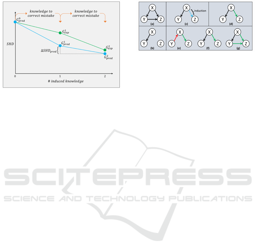
Figure 1: Knowledge induction process. We induce knowl-

edge by carrying over the existing knowledge set along with

a new random correction informed by model mistakes.

3 KNOWLEDGE INDUCTION

In our formulation, we use the multilayer perceptrons

of NOTEARS-MLP proposed by (Zheng et al., 2020)

as our estimators. We extend this framework to incor-

porate causal knowledge by characterizing the extra

information as additional constraints in the optimiza-

tion in Eq. 3.

Knowledge Type. We distinguish between these

two types of knowledge: (i) known inactive is knowl-

edge from the true inactive edges (absence of direct

causal relation), and (ii) known active is knowledge

from the true active edges (presence of direct causal

relation).

Knowledge Induction Process. We adopt an inter-

active induction process, where the expert knowledge

is informed by the outcome of the causal discovery

model. Namely, the knowledge is induced to correct

the mistakes of the model in the causal structure, in

the hope that the new structure is closer to the true

causal graph. This process is applied sequentially by

correcting the mistakes of the model at each step.

In the following subsections we present the formu-

lation of the NOTEARS optimization with constrains

and detail the sequential induction process.

3.1 Expert Knowledge as Constraints

An induced knowledge associated with a true ac-

tive edge, X

→ X

(known active) enforces the cor-

responding cell in the adjacency matrix to be non-

zero, [W (θ)]

i j

̸= 0. We consider this knowledge as

Figure 2: Expected graph formulation: (a) true graph, G

true

(b) predicted graph by model at step k, G

pred

, (c) induced

knowledge at step (k +1), (d) expected graph at step (k+1),

k+1

exp

. Three different examples of many possible predicted

graphs at step (k + 1), G

k+1

pred

where the model performs (e)

less than expectation, (f) par with expectation, and (g) more

than expectation.

inequality constraint in our extension of the optimiza-

tion such that the following statement holds:

ineq

(W (θ)) > 0

(5)

where p enumerates over all the inequality constraints

due to induction from the set of known active and

ineq

is the penalty score associated with the viola-

tion of these inequality constraints. On the other

hand, knowledge associated with true inactive edge,

↛ X

(known inactive) enforces the related cell in

W (θ) to be equal to zero, [W (θ)]

i j

= 0 if the induction

implies there should not be an edge from X

to X

. We

consider this knowledge as equality constraint in our

optimization such as:

(W (θ)) = 0

(6)

where q enumerates over all the equality constraints,

induced from the set of known inactive and h

is the

penalty score associated with the violation of these

equality constraints. With these additional constraints

in Eqs. 5, 6 we extend Eq. 3 to incorporate causal

knowledge in the optimization as follows:

min

f : f

∈H

),∀ j∈[d]

L( f )

subject to h(W (θ)) = 0,

(W (θ)) = 0,

ineq

(W (θ)) > 0

(7)

NOTEARS uses a thresholding step on the estimated

edge weights to reduce false discoveries by pruning

all the edges with weights falling below a certain

threshold. Because of this, in practice, even the equal-

ity constraints in Eq. 6 become inequalities to allow

for small weights. Finally, slack variables are intro-

duced in the implementation to transform the inequal-

ity constraints into equality constraints (see detailed

formulation in Appendix A).

Evaluation of Induced Expert Knowledge in Causal Structure Learning by NOTEARS

139

By using the similar strategy suggested by Zheng

et al. (Zheng et al., 2020) with augmented Lagrangian

method the reframed constrained optimization of

Eq. 4 takes the following form:

min

F(θ) + λ||θ||

F(θ) = L(θ) +

|h(W (θ))|

+ αh(W (θ))

∑

(

ineq

(W (θ))|

+ α

ineq

(W (θ)))

∑

(

(W (θ))|

+ α

(W (θ)))

(8)

3.2 Sequential Knowledge Induction

In case of knowledge induction, the optimization is

run in a sequential manner where the constraints are

informed by the causal mistakes made by the model

in the previous step. We start with our baseline model

without imposing any additional knowledge from the

true DAG and get the predicted causal graph denoted

by G

pred

in Figure 1. Then at each iterative step

(k + 1), based on the mistakes in the causal graph

pred

predicted by the NOTEARS-MLP, we select

one additional random piece of knowledge to correct

one of the mistakes, and add it to the set of con-

straints identiﬁed in the previous k steps, and rerun

NOTEARS. We note that a batch of corrections can

also be selected, however for this work we have fo-

cused on estimating the contribution of each piece of

knowledge in the form of known active/inactive edge.

Our observations are illustrated in Section 4.1, Sec-

tion 4.2, Section 4.3, and Section 4.4.

Expected Causal Graph. We consider the ex-

pected causal graph, G

k+1

exp

at step (k+1) by consider-

ing the case where all the knowledge has successfully

been induced without impacting any other edges. Fig-

ure 2d illustrates an example of how we formulate

our expected graph for a particular step in the itera-

tive process. We note that the correction might yield

a directed graph (Expected Causal Graph) that is not

necessary a DAG. The objective is to compare the

performance between the causal graph predicted by

NOTEARS and the expected causal graph. Our intu-

ition is that the induced knowledge will probably cor-

rect additional incorrect edges, see Figure 2g, yield-

ing a performance better than expected.

Table 1: Performance metrics considered with their corre-

sponding desirability.

Metric Desirability

∆FDR Lower is better

∆TPR Higher is better

∆FPR Lower is better

∆SHD Lower is better

Table 2: Results for inducing redundant knowledge.

Metric Mean ± Stderr. Remarks

∆FDR -0.00030 ± 0.00017 No harm

∆TPR -0.00035 ± 0.00027 No harm

∆FPR -0.00097 ± 0.00059 No harm

∆SHD -0.00154 ± 0.00167 No harm

4 EXPERIMENTS

To empirically evaluate the impact of additional

causal knowledge on causal learning and to keep our

experimental setup similar to the study in Ref. (Zheng

et al., 2020), we have used an MLP with 10 hid-

den units and sigmoid activation functions. In all our

experimental setup, we assume the prior knowledge

is correct (agrees with the true DAG). Despite the

known sensitivity of the NOTEARS algorithm to data

scaling, as demonstrated in previous study (Reisach

et al., 2021), we have conducted experiments using

both unscaled and scaled data to ensure the robustness

of our ﬁndings and we are pleased to report that our

conclusions remain unchanged regardless of the scal-

ing of the data, indicating the stability and reliability

of our results. While we present the results using the

unscaled data for consistency with the original imple-

mentation of NOTEARS (Zheng et al., 2020), it is

important to note that our conclusions hold true even

when the data is scaled.

Simulation. We investigate the performance of our

formulation and the impact of induced knowledge by

comparing the DAG estimates with the ground truths.

For our simulations with synthetic data, we have con-

sidered 16 different combinations following the sim-

ulation criteria: two random graph models, Erdos-

Renyi (ER) and Scale-Free (SF), number of nodes,

d = {10, 20}, sample size, n = {200, 1000}, edge

density, s0 = {1d, 4d}. For each of these combina-

tions, we have generated 10 different random graphs

or true DAGs (as 10 trials for a particular combina-

tion) and corresponding data by following nonlinear

data generating process with index models (similar

to the study in Ref. (Zheng et al., 2020) for which

the underlying true DAGs are identiﬁable. The results

ICPRAM 2023 - 12th International Conference on Pattern Recognition Applications and Methods

140

Table 3: Results for inducing knowledge that corrects model’s mistake.

Metric Knowledge Mean ± Stderr. Improvement

∆FDR inactive -0.018 ± 0.002 Signiﬁcant

∆FDR active -0.008 ± 0.001 Signiﬁcant

∆TPR inactive -0.007 ± 0.003 Not signiﬁcant

∆TPR active 0.024 ± 0.003 Signiﬁcant

∆FPR inactive -0.023 ± 0.004 Signiﬁcant

∆FPR active -0.008 ± 0.003 Signiﬁcant

∆SHD inactive -0.032 ± 0.012 Signiﬁcant

∆SHD active -0.071 ± 0.011 Signiﬁcant

are summarized over all these 160 random true DAGs

and datasets. In our simulations, we have considered

the regularization parameter, λ = 0.01. We evaluate

the performance of causal learning based on the mean

and the standard error of different metrics. For sta-

tistical signiﬁcance analysis, we have used t-test with

α = 0.05 as the signiﬁcance level.

Metrics. For the comparative analysis, we consider

the following performance metrics: False Discovery

Rate (FDR), True Positive Rate (TPR), False Posi-

tive Rate (FPR), and Structural Hamming Distance

(SHD). However, since we are evaluating the perfor-

mance over all these 160 random graphs of varying

sizes, we consider Structural Hamming Distance per

node (SHD/d) as our SHD measure that scales with

the number of nodes (FDR, TPR, and FPR scale by

deﬁnition). To evaluate the impact of induced knowl-

edge, we calculate the differences in the metrics at

different steps (where we have different sizes of in-

duced knowledge set) and referred them as ∆FDR,

∆TPR, ∆FPR, and ∆SHD, see also Table 1. For ex-

ample, based on our model’s prediction we calculate

the impact of inducing one additional piece of knowl-

edge on the metric SHD (∆SHD

pred

) as follows:

∆SHD

pred

= SHD(G

k+1

pred

) − SHD(G

pred

)

(9)

Sanity Check - Redundant Knowledge Does no

Harm. As part of our sanity check, we investigate

the impact of induced knowledge that matches the

causal relationships successfully discovered by the

NOTEARS-MLP. Therefore, in this section, we con-

sider the set of edges that our baseline model cor-

rectly classiﬁes as our knowledge source. Here, we do

not distinguish between the edge types of our induced

knowledge (known inactive & active) since our goal

is to investigate whether having redundant knowl-

edge as additional constraints affects model’s perfor-

mance or not. The results are illustrated in Table 2.

Our empirical evaluation shows that adding redun-

dant knowledge does not deteriorate the performance

of NOTEARS-MLP. Our performed statistical test re-

ﬂects that the results after inducing the knowledge

from the correctly classiﬁed edge set are not statis-

tically different than the results from the model with-

out these knowledge inductions. However, we have

noticed that the performance gets worse with highly

regularized models. This is consistent with observa-

tions by Ng et al. (Ng et al., 2020) where sparse DAGs

result in missing some of the true active edges.

4.1 Knowledge that Corrects Model’s

Mistake

We ﬁrst investigate the role of randomly chosen

knowledge that corrects model’s mistake based on

the cause-effect relations of the true graph. There-

fore, in this case, we consider the set of misclassiﬁed

edges from the estimated causal graph as the knowl-

edge source for biasing the model. The results are

illustrated in Table 3. Our empirical result shows sta-

tistically signiﬁcant improvements whenever the in-

duced knowledge corrects misclassiﬁed edges in the

estimated causal graph except for the case of ∆TPR

with known inactive edges. However, this behavior is

not totally unexpected since knowledge from known

inactive edges helps to get rid of false discoveries or

false positives, which hardly have impact on true pos-

itives.

4.2 Known Inactive vs Known Active

In this subsection, we are interested in understanding

the impact of different types of induced knowledge

on causal discovery to correct the mistakes in the es-

timated causal graph. As a result, the experimental

setup is similar to Section 4.1 where we consider the

misclassiﬁed edge set as the knowledge source. We

consider both known inactive and known active types

of knowledge to induce separately and analyze the

differences of their impact on the performance. The

results are illustrated in Table 4. Based on our statis-

tical test, we have found that inducing known inactive

is more effective when we compare the performance

Evaluation of Induced Expert Knowledge in Causal Structure Learning by NOTEARS

141

Table 4: Comparison between the impact of inducing knowledge regarding inactive vs active edges.

Metric Inactive Active Better

∆FDR -0.019 ± 0.002 -0.008 ± 0.001 inactive

∆TPR -0.007 ± 0.003 0.024 ± 0.003 active

∆FPR -0.023 ± 0.004 -0.009 ± 0.004 inactive

∆SHD -0.033 ± 0.013 -0.072 ± 0.011 active

Table 5: Comparison between the empirical performance vs expectation.

Metric Knowledge Empirical Expected Remarks

∆FDR inactive -0.019 ± 0.002 -0.016 ± 0.002 No difference

∆FDR active -0.008 ± 0.001 -0.006 ± 0.001 No difference

∆TPR inactive -0.007 ± 0.003 -0.002 ± 0.003 No difference

∆TPR active 0.024 ± 0.003 0.022 ± 0.002 No difference

∆FPR inactive -0.023 ± 0.004 -0.021 ± 0.004 No difference

∆FPR active -0.009 ± 0.003 -0.007 ± 0.003 No difference

∆SHD inactive -0.033 ± 0.013 -0.047 ± 0.010 No difference

∆SHD active -0.072 ± 0.011 -0.056 ± 0.010 No difference

based on FDR and FPR as misclassiﬁcation of inac-

tive edges has more impact on these metrics. On the

other hand, the results show that inducing known ac-

tive is more effective on TPR as misclassiﬁcation of

active edges has more impact on this metric. Inter-

estingly, we have found that known active provides a

signiﬁcant improvement over known inactive in terms

of SHD. This can be attributed to the fact that the

induced knowledge based on the true inactive edge

(known inactive) between two random variables, i.e.

from X

to X

allows for two extra degrees of freedom

since it is still possible to have no edge at all or an ac-

tive edge from X

to X

. However, the induced knowl-

edge based on the true active edge doesn’t allow any

degrees of freedom. This type of knowledge is more

restraining for causal graph discovery and therefore

carries more information.

4.3 Empirical Performance vs

Expectation

In this subsection, we are interested in understand-

ing whether inducing knowledge to correct model’s

mistakes exceeds expected improvement. The ex-

perimental setup is similar to Section 4.1 and Sec-

tion 4.2 where we consider the misclassiﬁed edge set

as the knowledge source. We have conducted the ex-

periments using both known inactive and known ac-

tive types of knowledge separately. The expected

causal graph, G

exp

is formulated in a similar man-

ner described in Fig. 2. Table 5 shows the sum-

mary of the performance comparison in these cases

with the expected results. Our statistical test shows

that the induced correct knowledge does not cor-

rect on average more incorrect active and/or inactive

edges than expected. Therefore, using the informa-

tion from induced knowledge does not have addi-

tional impact than expected in the global optimiza-

tion scheme. However, this is likely due to the fact

that the structure of the expected causal graph, G

exp

is not well-posed. It’s worth noting that G

exp

isn’t

necessarily a DAG since there isn’t any constraining

mechanism to enforce acyclicity as compared to G

pred

(NOTEARS imposes hard acyclicity constaint in the

continuous optimization). Although it is to be noted

here that solving an acyclicity constrained optimiza-

tion problem does not guarantee to return a DAG and

Ng et al. (Ng et al., 2022) in their study illustrates on

this behavior and proposes the convergence guarantee

with a DAG solution.

4.4 Real Data

We evaluate the implication of incorporating expert

knowledge on the dataset from study in Ref. (Sachs

et al., 2005), which is largely used in the literature of

probabilistic graphical models with a consensus net-

work accepted by the biological community. This

dataset contains the expression levels of phosphory-

lated proteins and phospholipids in human cells under

different conditions. The dataset has d = 11 cell types

along with n = 7466 samples of expression levels. As

for the ground truth of the underlying causal graph,

we considered s

= 20 active edges as suggested by

the study (Sachs et al., 2005). We have opted for

∆TPR, the percentage difference of edges in agree-

ment (higher is better), and the percentage difference

of reversed edges (lower is better) as the evaluation

metrics since the performance on these metrics would

indicate the signiﬁcance more distinctively. Similar

ICPRAM 2023 - 12th International Conference on Pattern Recognition Applications and Methods

142

to the synthetic data analysis, we had 10 trials that

we used to summarize our evaluation. Our empiri-

cal result (Mean ± Stderr.) shows: ∆TPR as 0.020

± 0.004, the percentage difference of edges in agree-

ment as 0.393 ± 0.086, and the percentage difference

of reversed edges as -0.073 ± 0.030. We have found

that with the help of induced knowledge the model

shows statistically signiﬁcant improvement by cor-

rectly identifying more active edges and by reducing

the number of edges identiﬁed in the reverse direc-

tion. Due to the limitation of having access only to a

subset of the true active edges, our analyses could not

include a comparative study on known inactive edges

as in the synthetic data case. We assume the perfor-

mance could have been improved by ﬁne-tuning the

model’s parameters but since our main focus of this

study is entirely based on the analyses regarding the

impact of induced knowledge of different types and

from different sources on structure learning, we kept

the parameter setup similar for all consecutive steps

in the knowledge induction process.

5 CONCLUSIONS

We have studied the impact of expert causal knowl-

edge on causal structure learning and provided a set

of comparative analyses of biasing the model using

different types of knowledge. Our ﬁndings show that

knowledge that corrects model’s mistakes yields sig-

niﬁcant improvements and it does no harm even in the

case of redundant knowledge that results in redundant

constraints. This suggest that the practitioners should

consider incorporating domain knowledge whenever

available. More importantly, we have found that

knowledge related to active edges has a larger positive

impact on causal discovery than knowledge related to

inactive edges which can mostly be attributed to the

difference between the number of degrees of freedom

each case reduces. This ﬁnding suggest that the prac-

titioners may want to prioritize incorporating knowl-

edge regarding presence of an edge whenever appli-

cable. Furthermore, our experimental analysis shows

that the induced knowledge does not correct on av-

erage more incorrect active and/or inactive edges than

expected. This ﬁnding is rather surprising to us, as we

have expected that every constraint based on a known

active/inactive edge to impact and correct more than

one edge on average.

Our work points to the importance of the human-

in-the-loop in causal discovery that we would like to

further explore in our future studies. Also, we would

like to mention that in our study we adopted hard con-

straints to accommodate the prior knowledge since we

have assumed our priors to be correct. An interesting

future direction would be to accommodate the contin-

uous optimization with functionality to allow differ-

ent levels of conﬁdence on the priors.

ACKNOWLEDGEMENTS

Research was sponsored by the Army Research Of-

ﬁce and was accomplished under Grant Number

W911NF-22-1-0035. The views and conclusions con-

tained in this document are those of the authors and

should not be interpreted as representing the ofﬁcial

policies, either expressed or implied, of the Army

Research Ofﬁce or the U.S. Government. The U.S.

Government is authorized to reproduce and distribute

reprints for Government purposes notwithstanding

any copyright notation herein.

REFERENCES

Alrajeh, D., Chockler, H., and Halpern, J. Y. (2020). Com-

bining experts’ causal judgments. Artiﬁcial Intelli-

gence, 288:103355.

Andrews, B., Spirtes, P., and Cooper, G. F. (2020). On the

completeness of causal discovery in the presence of la-

tent confounding with tiered background knowledge.

In International Conference on Artiﬁcial Intelligence

and Statistics, pages 4002–4011. PMLR.

Bertsekas, D. P. (1997). Nonlinear programming. Journal

of the Operational Research Society, 48(3):334–334.

Bhattacharjya, D., Gao, T., Mattei, N., and Subramanian, D.

(2021). Cause-effect association between event pairs

in event datasets. In Proceedings of the Twenty-Ninth

International Conference on International Joint Con-

ferences on Artiﬁcial Intelligence, pages 1202–1208.

Bradley, R., Dietrich, F., and List, C. (2014). Aggregating

causal judgments. Philosophy of Science, 81(4):491–

515.

Chickering, D. M. (1996). Learning Bayesian networks is

NP-complete. In Learning from data, pages 121–130.

Springer.

Chickering, D. M. (2002). Optimal structure identiﬁcation

with greedy search. Journal of machine learning re-

search, 3(Nov):507–554.

Chickering, M., Heckerman, D., and Meek, C. (2004).

Large-sample learning of Bayesian networks is NP-

hard. Journal of Machine Learning Research, 5.

Colombo, D., Maathuis, M. H., Kalisch, M., and Richard-

son, T. S. (2012). Learning high-dimensional directed

acyclic graphs with latent and selection variables. The

Annals of Statistics, pages 294–321.

Cooper, G. (1995). Causal discovery from data in the pres-

ence of selection bias. In Proceedings of the Fifth

International Workshop on Artiﬁcial Intelligence and

Statistics, pages 140–150.

Evaluation of Induced Expert Knowledge in Causal Structure Learning by NOTEARS

143

Elkan, C. (2001). The foundations of cost-sensitive learn-

ing. In International joint conference on artiﬁcial in-

telligence, volume 17, pages 973–978. Lawrence Erl-

baum Associates Ltd.

Fang, Z., Zhu, S., Zhang, J., Liu, Y., Chen, Z., and He, Y.

(2020). Low rank directed acyclic graphs and causal

structure learning. arXiv preprint arXiv:2006.05691.

Gencoglu, O. and Gruber, M. (2020). Causal modeling

of twitter activity during Covid-19. Computation,

8(4):85.

Heindorf, S., Scholten, Y., Wachsmuth, H.,

Ngonga Ngomo, A.-C., and Potthast, M. (2020).

Causenet: Towards a causality graph extracted from

the web. In Proceedings of the 29th ACM Inter-

national Conference on Information & Knowledge

Management, pages 3023–3030.

Holzinger, A. (2016). Interactive machine learning for

health informatics: when do we need the human-in-

the-loop? Brain Informatics, 3(2):119–131.

Jaber, A., Zhang, J., and Bareinboim, E. (2018). Causal

identiﬁcation under Markov equivalence. arXiv

preprint arXiv:1812.06209.

Lachapelle, S., Brouillard, P., Deleu, T., and Lacoste-Julien,

S. (2019). Gradient-based neural DAG learning. arXiv

preprint arXiv:1906.02226.

Lake, B. M., Ullman, T. D., Tenenbaum, J. B., and Gersh-

man, S. J. (2017). Building machines that learn and

think like people. Behavioral and brain sciences, 40.

Li, Z., Ding, X., Liu, T., Hu, J. E., and Van Durme, B.

(2021). Guided generation of cause and effect. arXiv

preprint arXiv:2107.09846.

Liu, J., Chen, Y., and Zhao, J. (2021). Knowledge enhanced

event causality identiﬁcation with mention masking

generalizations. In Proceedings of the Twenty-Ninth

International Conference on International Joint Con-

ferences on Artiﬁcial Intelligence, pages 3608–3614.

Magliacane, S., van Ommen, T., Claassen, T., Bongers,

S., Versteeg, P., and Mooij, J. M. (2017). Do-

main adaptation by using causal inference to pre-

dict invariant conditional distributions. arXiv preprint

arXiv:1707.06422.

Ng, I., Fang, Z., Zhu, S., Chen, Z., and Wang, J.

(2019). Masked gradient-based causal structure learn-

ing. arXiv preprint arXiv:1910.08527.

Ng, I., Ghassami, A., and Zhang, K. (2020). On the role

of sparsity and DAG constraints for learning linear

DAGs. arXiv preprint arXiv:2006.10201.

Ng, I., Lachapelle, S., Ke, N. R., Lacoste-Julien, S., and

Zhang, K. (2022). On the convergence of continuous

constrained optimization for structure learning. In In-

ternational Conference on Artiﬁcial Intelligence and

Statistics, pages 8176–8198. PMLR.

O’Donnell, R. T., Nicholson, A. E., Han, B., Korb, K. B.,

Alam, M. J., and Hope, L. R. (2006). Causal discov-

ery with prior information. In Australasian Joint Con-

ference on Artiﬁcial Intelligence, pages 1162–1167.

Springer.

Pearl, J. (2009). Causality. Cambridge university press.

Pearl, J. and Verma, T. S. (1995). A theory of inferred cau-

sation. In Studies in Logic and the Foundations of

Mathematics, volume 134, pages 789–811. Elsevier.

Peters, J., Janzing, D., and Sch

olkopf, B. (2017). Elements

of causal inference: foundations and learning algo-

rithms. The MIT Press.

Ramsey, J., Glymour, M., Sanchez-Romero, R., and Gly-

mour, C. (2017). A million variables and more: the

Fast Greedy Equivalence Search algorithm for learn-

ing high-dimensional graphical causal models, with

an application to functional magnetic resonance im-

ages. International journal of data science and ana-

lytics, 3(2):121–129.

Reisach, A., Seiler, C., and Weichwald, S. (2021). Beware

of the simulated dag! causal discovery benchmarks

may be easy to game. Advances in Neural Information

Processing Systems, 34:27772–27784.

Sachs, K., Perez, O., Pe’er, D., Lauffenburger, D. A., and

Nolan, G. P. (2005). Causal protein-signaling net-

works derived from multiparameter single-cell data.

Science, 308(5721):523–529.

Scutari, M. (2009). Learning bayesian networks with the

bnlearn r package. arXiv preprint arXiv:0908.3817.

Sharma, A. and Kiciman, E. (2020). Dowhy: An end-

to-end library for causal inference. arXiv preprint

arXiv:2011.04216.

Spirtes, P., Glymour, C. N., Scheines, R., and Heckerman,

D. (2000). Causation, prediction, and search. MIT

press.

Wei, D., Gao, T., and Yu, Y. (2020). Dags with no fears:

A closer look at continuous optimization for learning

bayesian networks. arXiv preprint arXiv:2010.09133.

Xin, D., Ma, L., Liu, J., Macke, S., Song, S., and

Parameswaran, A. (2018). Accelerating human-in-

the-loop machine learning: Challenges and opportu-

nities. In Proceedings of the second workshop on data

management for end-to-end machine learning, pages

1–4.

Yang, Y., Kandogan, E., Li, Y., Sen, P., and Lasecki, W. S.

(2019). A study on interaction in human-in-the-loop

machine learning for text analytics. In IUI Workshops.

Yu, Y., Chen, J., Gao, T., and Yu, M. (2019). DAG-GNN:

DAG structure learning with graph neural networks.

In International Conference on Machine Learning,

pages 7154–7163. PMLR.

Zadrozny, B. (2004). Learning and evaluating classi-

ﬁers under sample selection bias. In Proceedings of

the twenty-ﬁrst international conference on Machine

learning, page 114.

Zhang, K., Zhu, S., Kalander, M., Ng, I., Ye, J., Chen, Z.,

and Pan, L. (2021). gcastle: A python toolbox for

causal discovery. arXiv preprint arXiv:2111.15155.

Zheng, X., Aragam, B., Ravikumar, P., and Xing, E. P.

(2018). DAGs with no tears: Continuous op-

timization for structure learning. arXiv preprint

arXiv:1803.01422.

Zheng, X., Dan, C., Aragam, B., Ravikumar, P., and Xing,

E. (2020). Learning sparse nonparametric DAGs.

In International Conference on Artiﬁcial Intelligence

and Statistics, pages 3414–3425. PMLR.

ICPRAM 2023 - 12th International Conference on Pattern Recognition Applications and Methods

144

APPENDIX

We illustrate here the detailed performance with sum-

mary statistics of induced knowledge from our em-

pirical evaluation (∆FDR, ∆TPR, ∆FPR, and ∆SHD

for both ∆=1 and ∆=2). Similar to one additional

knowledge (∆=1), we calculate the impact of induc-

ing two additional piece of knowledge (∆=2) based

on our model’s prediction i.e. on the metric SHD

(∆SHD

pred

) as follows:

∆SHD

pred

= SHD(G

k+2

pred

) − SHD(G

pred

)

(10)

Table 6 shows the results for inducing redundant

knowledge or knowledge that is correctly classiﬁed

by NOTEARS-MLP.

A. Threshold Incorporation and Slack Variables.

In Eq. 5, we have seen that our inequality constraint

takes the following form:

ineq

(W (θ)) > 0

where p enumerates over each induced knowledge as-

sociated with true active edge (known active) X

→ X

imposing [W (θ)]

i j

̸= 0. NOTEARS uses a threshold-

ing step that reduces false discoveries where any edge

weight below the threshold value, w

thresh

in its ab-

solute value is set to zero. Thus, for any induction

from true active edges (X

→ X

) we have the follow-

ing constraint:

[W (θ)]

i j

≥ W

thresh

We convert inequality constraints in our optimization

to equality by introducing a set of slack variables y

such that:

− [W (θ)]

i j

thresh

+ y

= 0 s.t. y

≥ 0

(11)

In a similar manner, using the threshold value,

thresh

our equality constraints (associated with

known inactive edges) take the form as:

[W (θ)]

i j

−W

thresh

+ y

= 0 s.t. y

≥ 0

(12)

where q enumerates over each induction asso-

ciated with true inactive edge X

↛ X

imposing

[W (θ)]

i j

= 0.

B. Additional Results and Summary Statistics.

Table 7 shows the detailed results for inducing knowl-

edge that corrects model’s mistake. Table 8 shows the

Table 6: Full results for inducing redundant knowledge (Sanity Check).

Metric ∆ Mean ± Stderr. p-value t-stat Remarks

∆FDR 1 -0.00030 ± 0.00017 0.076 -1.770 No harm

∆FDR 2 -0.00060 ± 0.00021 0.004 -2.850 No harm

∆TPR 1 -0.00035 ± 0.00027 0.205 -1.260 No harm

∆TPR 2 -0.00036 ± 0.00029 0.227 -1.210 No harm

∆FPR 1 -0.00097 ± 0.00059 0.100 -1.630 No harm

∆FPR 2 -0.00183 ± 0.00069 0.008 -2.660 No harm

∆SHD 1 -0.00154 ± 0.00167 0.356 -0.920 No harm

∆SHD 2 -0.00357 ± 0.00188 0.050 -1.900 No harm

Table 7: Full results for inducing knowledge that corrects model’s mistake (Section 4.1).

Metric ∆ Knowledge Mean ± Stderr. p-value t-stat Improvement

∆FDR 1 inactive -0.018, 0.002 3.41E-14 -7.800 Signiﬁcant

∆FDR 1 active -0.008, 0.001 2.51E-08 -5.657 Signiﬁcant

∆FDR 2 inactive -0.023, 0.003 2.74E-15 -8.221 Signiﬁcant

∆FDR 2 active -0.011, 0.002 9.06E-08 -5.448 Signiﬁcant

∆TPR 1 inactive -0.007, 0.003 3.10E-02 -2.164 Not signiﬁcant

∆TPR 1 active 0.024, 0.003 8.58E-19 9.191 Signiﬁcant

∆TPR 2 inactive -0.001, 0.003 8.25E-01 -0.222 Not signiﬁcant

∆TPR 2 active 0.035, 0.004 1.16E-19 9.580 Signiﬁcant

∆FPR 1 inactive -0.023, 0.004 3.81E-08 -5.583 Signiﬁcant

∆FPR 1 active -0.008, 0.003 1.21E-02 -2.517 Signiﬁcant

∆FPR 2 inactive -0.021, 0.003 1.04E-08 -5.845 Signiﬁcant

∆FPR 2 active -0.015, 0.005 6.73E-03 -2.724 Signiﬁcant

∆SHD 1 inactive -0.032, 0.012 9.74E-03 -2.594 Signiﬁcant

∆SHD 1 active -0.071, 0.011 1.61E-10 -6.522 Signiﬁcant

∆SHD 2 inactive -0.082, 0.012 1.93E-10 -6.533 Signiﬁcant

∆SHD 2 active -0.126, 0.016 3.41E-14 -7.875 Signiﬁcant

Evaluation of Induced Expert Knowledge in Causal Structure Learning by NOTEARS

145

Table 8: Full results of comparison between the impact of inducing knowledge regarding inactive vs active edges. (Sec-

tion 4.2).

Metric ∆ Inactive Active p-value t-stat Better

∆FDR 1 -0.019 ± 0.002 -0.008 ± 0.001 1.30E-04 -3.85 Inactive

∆FDR 2 -0.023 ± 0.002 -0.011 ± 0.001 5.58E-04 -3.47 Inactive

∆TPR 1 -0.007 ± 0.003 0.024 ± 0.003 8.13E-14 -7.57 Active

∆TPR 2 -0.001 ± 0.003 0.035 ± 0.004 2.84E-13 -7.43 Active

∆FPR 1 -0.023 ± 0.004 -0.009 ± 0.004 7.28E-03 -2.69 Inactive

∆FPR 2 -0.021 ± 0.004 -0.015 ± 0.005 3.23E-01 -0.99 No difference

∆SHD 1 -0.033 ± 0.013 -0.072 ± 0.011 1.90E-02 2.35 Active

∆SHD 2 -0.082 ± 0.013 -0.126 ± 0.016 3.28E-02 2.14 Active

Table 9: Full results of comparison between the empirical performance vs expectation (Section 4.3).

Metric ∆ Knowledge Empirical Expected p-value t-stat Remarks

∆FDR 1 inactive -0.019 ± 0.002 -0.016 ± 0.002 0.51 -0.65 No difference

∆FDR 1 active -0.008 ± 0.001 -0.006 ± 0.001 0.21 -1.25 No difference

∆FDR 2 inactive -0.023 ± 0.002 -0.025 ± 0.002 0.60 0.53 No difference

∆FDR 2 active -0.011 ± 0.002 -0.010 ± 0.002 0.75 -0.32 No difference

∆TPR 1 inactive -0.007 ± 0.003 -0.002 ± 0.003 0.22 -1.23 No difference

∆TPR 1 active 0.024 ± 0.003 0.022 ± 0.002 0.48 0.70 No difference

∆TPR 2 inactive -0.001 ± 0.003 -0.006 ± 0.003 0.24 1.17 No difference

∆TPR 2 active 0.035 ± 0.004 0.028 ± 0.004 0.18 1.34 No difference

∆FPR 1 inactive -0.023 ± 0.004 -0.021 ± 0.004 0.62 -0.50 No difference

∆FPR 1 active -0.009 ± 0.003 -0.007 ± 0.003 0.79 -0.27 No difference

∆FPR 2 inactive -0.021 ± 0.004 -0.030 ± 0.005 0.18 1.34 No difference

∆FPR 2 active -0.015 ± 0.005 -0.018 ± 0.005 0.61 0.51 No difference

∆SHD 1 inactive -0.033 ± 0.013 -0.047 ± 0.010 0.36 0.91 No difference

∆SHD 1 active -0.072 ± 0.011 -0.056 ± 0.010 0.30 -1.04 No difference

∆SHD 2 inactive -0.082 ± 0.013 -0.086 ± 0.013 0.82 0.23 No difference

∆SHD 2 active -0.126 ± 0.016 -0.100 ± 0.017 0.28 -1.09 No difference

Table 10: Full results for inducing knowledge in real data (Section 4.4).

Metric ∆ Mean ± Stderr. p-value t-stat Remarks

∆TPR 1 0.020 ± 0.004 8.10E-06 4.60 Improvement

∆TPR 2 0.036 ± 0.005 1.77E-12 7.62 Improvement

∆ % edge in agreement 1 0.393 ± 0.086 8.10E-06 4.60 Improvement

∆ % edge in agreement 2 0.714 ± 0.094 1.77E-12 7.62 Improvement

∆ % edge reversed 1 -0.073 ± 0.030 1.54E-02 -2.45 Improvement

∆ % edge reversed 2 -0.107 ± 0.033 1.29E-03 -3.27 Improvement

detailed results of the difference between the impact

of ‘known inactive’ (knowledge induced from inac-

tive edges) and ‘known active’ (knowledge induced

from active edges) using misclassiﬁed edge set as the

knowledge source. Table 9 shows the detailed re-

sults of the difference between empirical improve-

ments due to knowledge induction vs expected out-

comes using misclassiﬁed edge set as the knowledge

source. Table 10 shows the detailed results for induc-

ing knowledge on the real dataset (from (Sachs et al.,

2005)).

ICPRAM 2023 - 12th International Conference on Pattern Recognition Applications and Methods

146