Integration of Efﬁcient Deep Q-Network Techniques Into QT-Opt

Reinforcement Learning Structure

Shudao Wei

, Chenxing Li

1,2

, Jan Seyler

and Shahram Eivazi

1,2

Department of Computer Science, University of T

ubingen, T

ubingen, Germany

Advanced Develop. Analytics and Control, Festo SE and Co. KG, Esslingen, Germany

Keywords:

Prioritized Experience Replay, Noisy Network, Mixed Policy, Distributed Reinforcement Learning,

Q-Function Targets Via Optimization, Quantile Q Target Optimizer.

Abstract:

There has been a growing interest in the development of ofﬂine reinforcement learning (RL) algorithms for

real-world applications. For example, ofﬂine algorithms like qt-opt has demonstrated an impressive perfor-

mance in grasping task. The primary motivation is to avoid the challenges associated with online data col-

lection. However, these algorithms require extremely large dataset as well as huge computational resources.

In this paper we investigate the applicability of well known improvement techniques from Deep Q-learning

(DQN) methods to the QT-Opt ofﬂine algorithm, for both on-policy and mixed-policy training. For the ﬁrst

time, we show that prioritized experience replay(PER), noisy network, and distributional DQN can be used

within QT-Opt framework. As result,for example, in a reacher environment from Pybullet simulation, we

observe an obvious improvements in the learning process for the integrated techniques.

1 INTRODUCTION

For many years, reinforcement learning (RL) has re-

ceived extensive attention, designed to describe and

solve problems, in which agents learn strategies to

achieve speciﬁc goals while interacting with the en-

vironment. Recently, RL has had fair achievements

in real-world applications as such the implementa-

tion of more speciﬁc real-world applications requires,

RL’s learning efﬁciency become the goal to pursue.

Given the vision-based data scope, the single-step du-

ration and memory footprint required for training an

agent are much more extensive than a value-based

task. How to solve tasks in larger-scale environments

with as few data and training steps as possible has be-

come a focus of attention in RL.

A leading example for large scale real-world prob-

lem is QT-Opt (Kalashnikov et al., 2018) (Q-function

Targets via Optimization) RL algorithm which is de-

signed to provide generalization for different tasks

and adaptation for compound action space. It meets

the demand with a distributed asynchronous structure,

a derivative-free optimization, and both online and of-

ﬂine training.

Main limitation of QT-Opt algorithms is that re-

quires extremely large dataset as well as huge com-

putational resources. To meet the demand for learn-

ing efﬁciency of RL in real-world in this paper we

propose to apply well-known rainbow (Hessel et al.,

2018) improvement techniques to the vanilla QT-Opt.

Hessel et al. (Hessel et al., 2018) empiri-

cally showed that prioritized experience replay(PER)

(Schaul et al., 2015), noisy network (Fortunato et al.,

2017), and distributional DQN (Bellemare et al.,

2017; Dabney et al., 2018b; Dabney et al., 2018a)

can improve overall performance of Deep Q-learning

(DQN) algorithm. Prioritized experience replay

(PER) (Schaul et al., 2015) in replay buffer sam-

ples training data non-uniformly under data potency,

which exploits the available data more effectively;

Noisy network (Fortunato et al., 2017) raises the ran-

domness from the action selection level to the net-

work level to generate new trajectory logic, which

stimulates more complex explorations; Q-value in

distributional perspective (Bellemare et al., 2017;

Dabney et al., 2018b; Dabney et al., 2018a) provides

more comprehensive information for action selection.

To our knowledge, there is no studies combin-

ing rainbow improvements in qt-opt structure. In

this paper we implement these techniques in away

to be compatible with non-distribution version of qt-

opt. We conduct separate and integrated experiments

in the vector-based robotic environments to provide

baselines in the centralized PyBullet (Coumans and

592

Wei, S., Li, C., Seyler, J. and Eivazi, S.

Integration of Efﬁcient Deep Q-Network Techniques Into QT-Opt Reinforcement Learning Structure.

DOI: 10.5220/0011715000003393

In Proceedings of the 15th International Conference on Agents and Artiﬁcial Intelligence (ICAART 2023) - Volume 3, pages 592-599

ISBN: 978-989-758-623-1; ISSN: 2184-433X

 2023 by SCITEPRESS – Science and Technology Publications, Lda. Under CC license (CC BY-NC-ND 4.0)

Bai, 2021) simulated environments. Our contribution

lists as follows:

• Benchmark of the QT-Opt performance under dif-

ferent basic robotic value-based environments.

• Attempts of PER Noisy network integration to-

gether with QT-Opt and distributional DQN (Q2-

Opt), with the purpose to pursue training efﬁ-

ciency.

In this paper, we ﬁrst introduce the current status

and related work. Then the fundamentals of learn-

ing techniques and our methods are demonstrated. Fi-

nally, the experiments are analysed and compared.

2 RELATED WORKS

Reinforcement learning (RL) from a model-free per-

spective Q-Learning (Watkins and Dayan, 1992) is an

algorithm that optimizes the action state value (Q-

value) by iterative function repeatedly. To solve the

exponential explosion of the action dimension, Deep

Q-Learning (DQN) (Li, 2017) has been proposed,

which approximates the q-value function by a deep

neural network. Double Q-learning(Hasselt, 2010)

algorithm was proposed, which utilizes two value

functions to separate action selection and state eval-

uation processes to exclude the maximization pro-

cess from the state evaluation. From this the dou-

ble DQN (Van Hasselt et al., 2016) is derived, which

maintains the separate state-action value evaluation

network with an update delay, leveraging the target

q-network from the original DQN. Clipped Double

DQN (Fujimoto et al., 2018) is an extension algo-

rithm to DQN, designed to address Q-value bias aris-

ing from the inherent estimation errors in Q-learning.

Cross-Entropy Method (CEM) (De Boer et al.,

2005; Kalashnikov et al., 2018) replace the maxi-

mization process in action selection by a stochastic

optimization over the actions. CEM is simple to im-

plement, has robust properties around local optima in

low-dimension problems, and no derivative operation,

thus it is ideal for RL algorithms. QT-Opt (Kalash-

nikov et al., 2018) employed both Clipped double

DQN and CEM to reduce the possible overestimation

of the q-value. Furthermore, it provides a distributed

asynchronous structure to achieve parallel training of

one agent network.

Based on distributional DQN technique, the same

team presented Q2-Opt(Bodnar et al., 2020), which

changes the q-value to the q-distribution and repre-

sents the action state relation more comprehensively.

Q2-Opt (Bodnar et al., 2020) is a distributional vari-

ant of QT-Opt. Two sub-versions of this enhance-

ment are provided: Q2R-Opt based on Quantile-

Regression DQN (QR-DQN) and Q2F-Opt based on

Implicit Quantile Network (IQN). In the QR-DQN

the p-Wasserstein metric (Vaserstein, 1969, 64–72.)

replacing the KL-divergence is utilized to describe

the difference between two distributions. A Wasser-

stein metric considers not merely the probability of

the outcome events. The distance between them is

also important. It is more appropriate to the q-value

distribution since we concern more about the under-

lying similarity of the two distributions than match-

ing their likelihoods exactly. To minimize the p-

Wasserstein distance, the distributional Bellman up-

date is projected onto a parameterized quantile dis-

tribution over the set of quantile midpoints. Then it

utilizes the Quantile regression method (Koenker and

Hallock, 2001) for an unbiased stochastic approxima-

tion of the distribution. Since the quantile regres-

sion loss is not derivable at zero, a quantile Huber-

Loss(Dabney et al., 2018b) operates as the loss func-

tion in QR-DQN, given τ ∈ [0, 1] as the selected quan-

tile. QR-DQN could regulate its range of return value

without projection support. The number of atoms in

the quantile distribution is also manually adjustable.

IQN (Dabney et al., 2018a) is similar to QR-DQN

in which IQN also return a parameterized quantile

distribution. However, instead of the ﬁxed τ in QR-

DQN, the result in IQN is over a randomly generated

τ ∼ U([0, 1]) distorted by a distortion risk measure

β : [0, 1] → [0, 1]. The basic network structure of Q2-

Opt is similar to Figure 1 in the DNN Model block.

A signiﬁcant improvement has been made by this ex-

tension as shown in (Bodnar et al., 2020, Results).

In this paper we do not have a preference for risk

management, thus we only use the basic risk matrix

β(τ) = τ in Q2F-Opt. The correlation between risk

distortion and other improvements could be tested in

future works. For the CEM in Q2-Opt, it maximizes

the score mapped from distribution vector q which is

the output of the network.

To help achieve higher performance various re-

search groups focus on improving the structural com-

position perspective of RL. For instance, Prioritized

experience replay (PER) presented by Schaul, Tom,

et al. (Schaul et al., 2015), and Noisy network sug-

gested by M. Fortunato et al. (Fortunato et al.,

2017). PER prioritizes the experience in the replay

buffer to increase agents’ learning efﬁciency based

on data efﬁciency enhancement and data correlations

during training provided by the original replay buffer

structure. On the other hand, the noisy network is

aimed at exploration by attaching noise to network

weights instead of action selection, which has the pur-

pose to change consistent, potentially complex, state-

Integration of Efﬁcient Deep Q-Network Techniques Into QT-Opt Reinforcement Learning Structure

593

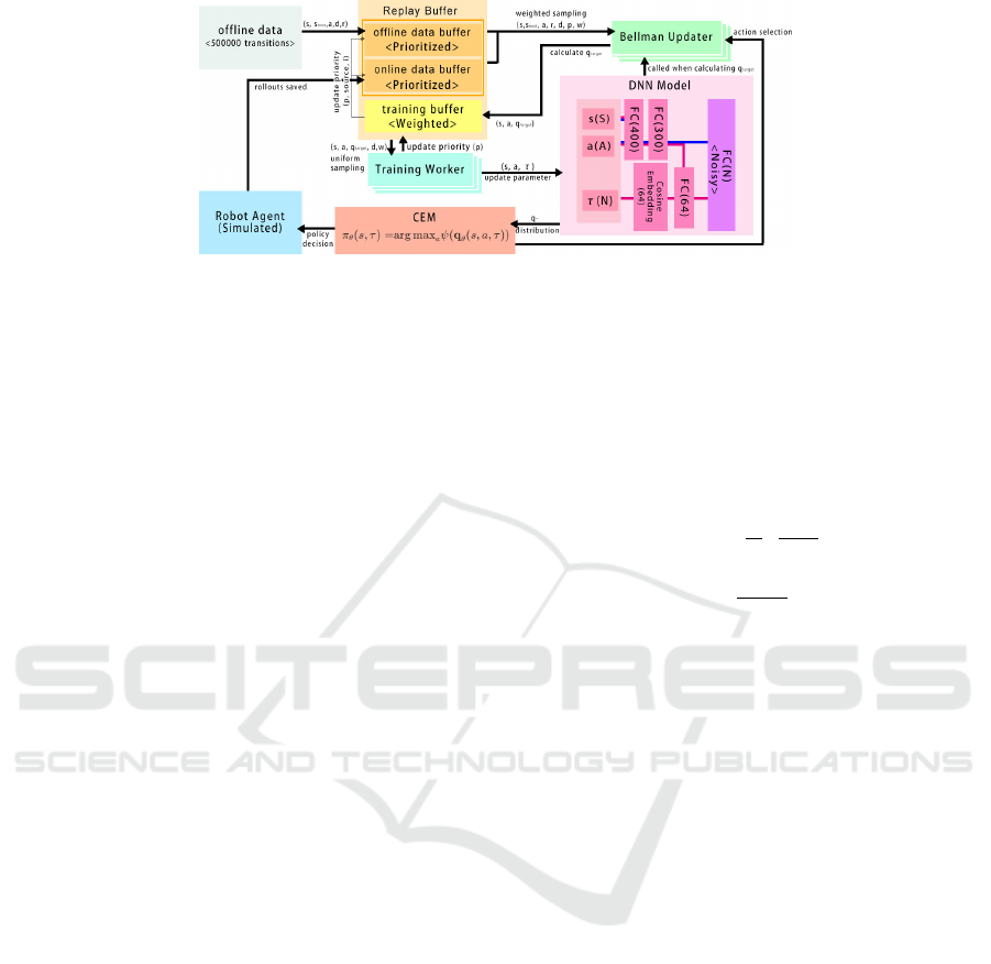
Figure 1: System architecture of our implementation of the extensions based on Q2-Opt. The rollouts simulated in the

environment are saved in the replay buffer after each 32-gradient update. The transitions from both data buffers are sampled

non-uniformly to the Bellman Updater, which appends the target q-distributions and is pushed to the training buffer which

could be asynchronously consumed by Training workers to compute the gradients. The parameters in the model deep neural

network are updated by gradient descent. Notice the lines in the DNN Model block, the pink line links the structure of

Q2R-Opt and the blue line links the structure of Q2F-Opt.

dependent behavior patterns. Our focus is also these

two techniques together with the distributed DQN ap-

proach, applied on Q2-Opt, which have been success-

fully applied in rainbow (Hessel et al., 2018) paper

for basic DQN algorithms.

3 METHODOLOGY

Figure 1 shows the architecture of our implementation

of the QT-Opt algorithm which has ﬁve main blocks:

replay buffer, Bellman updater, training worker, DNN

model, and CEM. Our modiﬁcations are mainly on

replay buffer and DNN Model blocks, while other

blocks merely attached several adaptions. With the

same operation process as vanilla QT-Opt described

in the preliminary section, our system run in single

computing machine compare to distributed version.

Moreover, we also implemented Q2-Opt based on the

description in (Bodnar et al., 2020).

3.1 Prioritized Replay

For an experience replay priority method extension

to QT-Opt, the data structure in the replay buffer is

replaced by a sum-segment-tree (Berg et al., 1997).

The priority value is set as the node value in the tree

structure. Considering the replay buffer structure in

QT-Opt, the PER method could be implemented in

data- or training buffer or both.

The sampling process in a prioritized replay buffer

started by uniformly sampling a batch of random val-

ues in the range [0,1). With the random batch mul-

tiplies by a sum over all priorities, we could use the

retrieve function in the sum-segment tree to get the

batch of the ﬁnal sampled index. The transitions are

picked from the buffer and sent together with the in-

dex and corresponding weights calculated by corre-

sponding priority as in the ensuing Equation, where

is the priority of i-th transition in the buffer:

= (

P (i)

)

(1)

P (i) =

∑

(2)

In our implementation, data buffer prioritization is

a conversion from the original PER deﬁnition: using

segment trees for importance sampling, picking out

and updating the transition data by indices. For train-

ing buffer, it is more complex. The training buffer

has to save the data source and corresponding in-

dices whether prioritized or not since we need to up-

date the priority value into the original on- or ofﬂine

data buffer together with the Bellman update. Priority

values are updated after each training batch and the

IS weight should be recalculated in each mini-batch.

Therefore, the training buffer also needs to calculate

the current weight with the locally updated priority

buffer if the gradient update per Bellman-update (gpb)

is larger than 1. To simplify the process we ﬁxed gpb

as 1 in our experiments.

Under the circumstances, in which the training

buffer is not prioritized, the sample weights are from

the data buffer importance sampling while Bellman

updating. We created a replay buffer subclass for this

kind of training buffer, which saves the corresponding

additional features and split the priority update batch

for two data buffers. If prioritized, the sample weights

are calculated from the training buffer itself. In other

words, when both types of buffers are prioritized,

our implementation is not saving the sample weights

from the data buffer, only sampling non-uniformly.

To update the priority which also adapts to distribu-

tional q-network results, considering the suggestion

ICAART 2023 - 15th International Conference on Agents and Artiﬁcial Intelligence

594

in Rainbow paper (Hessel et al., 2018, ’The Integrated

Agent’), we are using the element-wise loss value as

the priority. Two hyper-parameters are needed in the

PER: α is denoted as the prioritization scale, which is

ﬁxed as 0.5 in our training. β determines the decay of

probabilities, which is ﬁxed as linearly growing from

0.4 to 1 as suggested.

3.2 PAL

Regarding the time penalty and RAM consumption

with importance sampling, due to the segment-sum-

tree, making PAL(Fujimoto et al., 2020) as an alterna-

tive to PER is worth considering. As a mirrored loss

function of LAP(Fujimoto et al., 2020), PAL has an

equivalent expected gradient to a non-uniformly sam-

pled replay buffer using importance sampling to avoid

its bias. In other words, PAL is a loss function alter-

native to a prioritized replay buffer implementation.

We integrated PAL to QT-Opt by adding an alter-

native loss function instead of Huber-Loss or MSE.

While adapting to the q-distribution network, we

change the loss function in the original Q2-Opt by re-

placing the Huber-loss in ρ with PAL-loss. The ﬁnal

loss function for PAL attached Q2-Opt is as shown in

Equation 3.

PAL

(u) =











|δ

T D−Error

if |δ

T D−Error

| ≤ κ

|δ

T D−Error

α+1

α + 1

otherwise

λ =

∑

max(|δ

T D−Error

( j)|, 1)

(u) = |τ − I

T D−E rror

| · L

PAL

(δ

T D−Error

) (3)

x<0



1 x < 0

0 x ≥ 0

(Dabney et al., 2018b; Fujimoto et al., 2020) The def-

inition of the One hyper-parameter is needed in this

improvement implementation: α as in PER. In our

experiments, the value is ﬁxed at 0.5.

3.3 Noisy Nets

A noisy layer is appended after the feature network

and other extension implementations, as the ﬁnal out-

put layer. In our experiments, a noisy dense layer is

deﬁned as a subclass of standard linear dense layer,

adding µ

, µ

, σ

as trainable variables, and gen-

erating ε

, ε

as random variables. As shown in the

original paper (Fortunato et al., 2017), the function

realized by the fully connected noisy linear layer is:

y = (µ

+ σ

 ε

)x + (µ

+ σ

 ε

) (4)

Figure 2: Evaluation reward as a function of the training

time-step on ReacherBulletEnv-v0 environment. The data

is collected from on-policy training results. The plot on

the top shows the training efﬁciency difference caused by

different training batch sizes and the bottom plot shows

the training efﬁciency difference caused by variant training

buffer sizes. All curves in the plot are trained with the same

random seed 0.

To generate random variables, we choose factor-

ized Gaussian noise as suggested in (Fortunato et al.,

2017) to reduce compute time. If we use independent

Gaussian noise, since we are using a single-thread qt-

opt-based agent, the computational overhead for our

network structure is too large for our computing re-

source.

Besides the implementation in the DNN-model,

we have to reset its noise every training step to ac-

tivate a noisy network. Thus we need to label all

noisy layers by network creation and call their reset

functions at every gradient step. As shown in Fig-

ure 1, in our implementation, when a noisy network

is on, the last layer in the current network is changed

into a noisy layer. One hyper-parameter is needed in

the noisy network, the initial standard deviation value

used by initializing the σ variables.

4 EXPERIMENT

We tested several improvement techniques for QT-

Opt, including PER, noisy network, and distributional

DQN. Simulation environments with continuous con-

trol tasks generated by PyBulletGym engine are used

in the training process. We used ReacherBulletEnv-v0

environment from the default setting as well as few

other robotic environments limited to time and com-

Integration of Efﬁcient Deep Q-Network Techniques Into QT-Opt Reinforcement Learning Structure

595

Figure 3: Evaluation reward as a function of the train-

ing time-step on ReacherBulletEnv-v0 environment. The

data of the top plot is collected from on-policy training

results and the data in the bottom plot is collected from

mixed-policy training results. All curves are from noisy at-

tached QT-Opt agents with different initial standard devia-

tions. The red, blue, green, and purple curves correspond to

an agent with an initial standard deviation equal to 0.005,

0.01, 0.001, and 0.05. All curves in the plot are averaged

by three separate runs with three different random seeds

(133156, 254306, 369070). The half-transparent area shows

the range between the max and min value at this time-step

in three runs.

puting power costs.

To evaluate the algorithm performance, we are us-

ing the reward value from the default tasks. One eval-

uation step is taken after each 2048 training time step.

For each evaluation, we run 10 tests with the tempo-

ral agent and collect the averaged reward value per

step. One test means a complete run until the task

is done or a maximum step (150 for ”Reacher” and

1000 for other environments) is reached. For repro-

ducibility of the results, random seeds are set for Ten-

sorFlow, NumPy, and gym environments. To ensure

the validity of the test, Three full pieces of the train-

ing run with different random seeds are taken for all

setups. The ﬁnal reward values are taken from the

average among three tests and the range (max and

min value among the three tests) are also saved. The

curves in the following plots have been smoothed by

a Savitsky-Golay ﬁlter with a window size equal to 15

and an order of 4. Ranges around the curve show the

range between max and min values over three tests,

both values are smoothed with the same ﬁlter.

Compared to pure on-policy training, we are pro-

viding mixed-policy training as explained in the origi-

nal QT-Opt paper (Kalashnikov et al., 2018). A mixed

policy starts by training with ofﬂine data sets and

keeps collecting online data for one training rollout

for each 32 training steps. The online data percentage

grows linearly from 0% to 50% in the ﬁrst 50% train-

ing iterations. The ofﬂine data used in mix-policy ex-

periments are generated by pure online training. All

500k transitions in the online data buffer after a full

training run (300k steps for Reacher, 1M for other en-

vironments) are saved, which are loaded afterwards

for a mixed training as ofﬂine data. No priority val-

ues are saved or passed on by creating a new ofﬂine

data buffer.

Firstly, we tuned our model with different train-

ing buffer sizes and training batch sizes, as shown

in Figure 2. For the training buffer, the closer to the

Bellman-update batch size the better result of the test

gets. The gradient update batch size is more straight-

forward: the larger it is, the better it gets, and it

reaches its limit depending on the training buffer size.

Therefore in the following experiments, we make the

training buffer size equal to the gradient update batch

size. Besides, in our case, we consider more of a

single QT-Opt rather than a distributed asynchronous

QT-Opt as our experiment target. So we set the train-

ing buffer as the same size as the Bellman-update

batch to provide a single model. Hence these three

sizes are selected equally in the following experi-

ments.

With noisy network standard variation value ini-

tialized differently, the result does not catch up to the

vanilla training with a explore probability of 0.02. But

with a speciﬁc standard deviation initial value, the

noisy network could reach a similar result. If the ini-

tial standard-deviation value is more than 0.05 or less

than 0.0001, the agent does not end up with a positive

reward. To see how this hyperparameter affects the

result and to choose the best for the rest of the train-

ing, we run a small test with 2/3 steps of full train-

ing for four different initial standard deviation values

within the range of 0.05 and 0.0001. Each value for

three times with inconsistent random seeds. The re-

sults are shown in Figure 3. The optimal initial val-

ues for on and mixed policy are different even though

they are trained with the same parameters and random

seeds. We use 0.01 for on-policy training and 0.05 in

mixed-policy training as the default initial standard

deviation value for a noisy network in the following

experiments.

From Figure 4, we can see that the PER tech-

niques have no progressive results compared to the

original QT-Opt algorithm with both policies on all

tested environments excluding ReacherBulletEnv-v0.

However, PER technique does not hurt the learn-

ing ability of the QT-Opt agents in any of the tasks.

ICAART 2023 - 15th International Conference on Agents and Artiﬁcial Intelligence

596

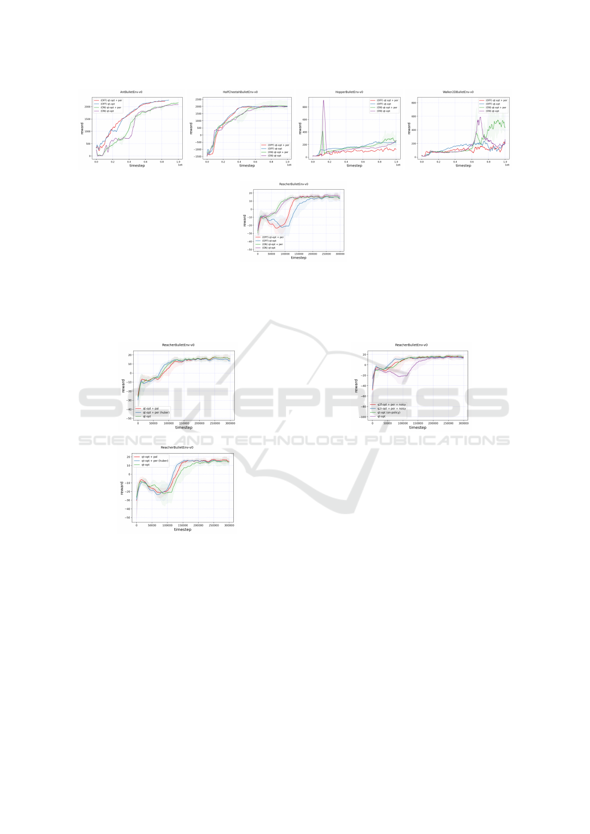
Figure 4: Evaluation reward as a function of the training time-step on AntBulletEnv-v0, HalfCheetahBulletEnv-v0,

HopperBulletEnv-v0, Walker2DBulletEnv-v0, and ReacherBulletEnv-v0 environment. The data is collected from mixed-policy

training results. The red curve is with PER attached QT-Opt agent trained in mixed-policy. The blue curve is with vanilla

QT-Opt agent trained in mixed-policy. The green curve is with PER attached QT-Opt agent trained in on-policy. The purple

curve is with the QT-Opt agent trained in on-policy. All curves in the other plots are averaged by three separate runs, while

all curves in the plot are trained with the same random seed.

Figure 5: Evaluation reward as a function of the training

time-step on ReacherBulletEnv-v0 environment. The data

in the top plot is collected from on-policy training results

and the data in the bottom plot is collected from mixed-

policy training results. The red curve is with PAL attached

QT-Opt agent. The blue curve is with PER attached QT-

Opt agent. The green curve is the vanilla QT-Opt agent. All

curves in the plot are averaged by three separate runs with

three different random seeds (133156, 254306, 369070).

The half-transparent area shows the range between the max

and min value at this time-step in three runs.

Notice that multi-pivot robot tasks have an obvi-

ous advantage in mixed-policy training in evalua-

tion rewards over on-policy training. However, in

the ReacherBulletEnv-v0 condition, it is the oppo-

Figure 6: Evaluation reward as a function of the training

time-step on ReacherBulletEnv-v0 environment. The data

is mainly collected from mixed-policy training results: The

blue curve is with PER and noisy attached Q2R-Opt agent,

the red curve is with PER and noisy attached Q2F-Opt

agent, and the purple curve is vanilla QT-Opt agent. Ex-

cept for the green curve, which is collected from on-policy

with vanilla QT-Opt agent. All curves in the plot are av-

eraged by three separate runs with three different random

seeds (133156, 254306, 369070). The half-transparent area

shows the range between the max and min value at this time-

step in three runs.

site. Additionally, in mixed-policy training, the PER-

attached QT-Opt agent has a more pronounced ef-

fect than the vanilla one. Therefore the follow-

ing experiments mostly proceed in mixed-policy.

For HopperBulletEnv-v0 and Walker2DBulletEnv-v0

tasks using humanoid robot structures, none of the

agents tend to a stabilized state.

As shown in Figure 5, PAL has almost as good

performance as PER in mixed-policy and could reach

a slightly higher ﬁnal mean reward. Compared to

the vanilla QT-Opt, both PAL and PER could provide

more learning efﬁciency. Meanwhile, with on-policy

tests, it performs even slower than vanilla QT-Opt.

Integration of Efﬁcient Deep Q-Network Techniques Into QT-Opt Reinforcement Learning Structure

597

Figure 7: Evaluation reward as a function of the training

time-step on ReacherBulletEnv-v0 environment. The data is

collected from mixed-policy training results. The red curve

is with noisy attached Q2F-Opt agent. The green curve is

with PER attached Q2F-Opt agent. The blue curve is with

PER and noisy attached Q2F-Opt agent. The purple curve

is with noisy attached Q2R-Opt agent. The yellow curve

is with PER attached Q2R-Opt agent. The orange curve is

with PER and noisy attached Q2R-Opt agent. All curves in

the plot are averaged by three separate runs with three dif-

ferent random seeds (133156, 254306, 369070). The half-

transparent area shows the range between the max and min

value at this time-step in three runs.

Considering its operational efﬁciency, PAL could be

a proper alternative to PER when no further changes

in loss function are required for an integrated agent.

Otherwise, it needs more theoretical proof for the un-

biasedness of the formula.

We begin with the ﬁnal results from the fully in-

tegrated agent, comparing with the performance of

vanilla QT-Opt. As shown in Figure 6, with both

PER and noisy network switched on as the base al-

gorithm, we add Q2-Opt techniques separately. We

found that Both Q2-Opt algorithms have better results

in mixed-policy tests, while comparing with the on-

policy vanilla QT-Opt they even maintains a proper

advantage. Comparing the results based on two Q2-

Opt variants, Q2R-Opt has better collaboration with

PER and noisy network methods regarding iteration

efﬁciency.

Then we evaluated the two techniques separated

and integrated on Q2-Opt as in Figure 7. Compared

to pure Q2R-Opt and pure Q2F-Opt, these two al-

gorithms attached with PER make a more obvious

efﬁciency increase than it has made in vanilla QT-

Opt. For Q2R-Opt, PER increases more with the as-

cent speed of learning, since the curve is steeper by

increasing. Meanwhile, for Q2F-Opt, PER only in-

creases the efﬁciency of the training steps by starting

the rewarding climb early. Its learning curve has al-

most the same, even more, gradual slope. We could

say that PER and Q2-Opt have good compatibility.

Meanwhile, noisy exploration on Q2R- and Q2F-Opt

speeds up the training by smoothing the learning at

the start, easily avoiding the slump in the beginning

but hardly being stable at around 50% of the time

steps. Noisy has a better correlation with Q2F-Opt,

but it also adds a large scale of instability to the eval-

uation results. So both PER and Noisy Network adds

to the base and could increase the speed of learn-

ing. When both of the techniques are switched on,

the learning curve could be increased furthermore.

Lastly, we extend the experiments with other

Pybullet simulated mujoco-like environments like

AntBulletEnv-v0, all the agents have demonstrated

their ability to learn and solve the tasks (Figure 8).

In these more complex environments, without hyper-

parameter tuning, PER and Q2-Opt variations do not

harm the learning abilities of the QT-Opt agent. How-

ever, these extensions could not overcome QT-Opt’s

weakness in humanoid-like robot ﬁelds.

5 DISCUSSION

In this paper, we have re-implemented the QT-Opt

and Q2-Opt (Kalashnikov et al., 2018; Bodnar et al.,

2020) algorithm with additional extension: PER

(Schaul et al., 2015) and Noisy network (Fortunato

et al., 2017) techniques. We conducted several exper-

iments separately on each extension to validate their

optimization effect on the algorithm, and proceed on

integrated tests combination of all techniques. More-

over, we tested use of PAL (Fujimoto et al., 2020)

instead of original PER. In the Reacher environment

by Pybullet simulation, we observe an obvious im-

provement in the learning process for a QT-Opt agent

with integrated methods. Meanwhile, in other related

robotic environments we conﬁrmed no harm in time-

step-efﬁciency when attaching these techniques on qt-

opt. Despite relatively considerable results, we still

observe few drawbacks with these extensions. First,

PER is not very cost-effective as an improvement to

QT-Opt, while PAL as its simplify equivalent have

lost most of the efﬁciency advantage. Second, the

Noisy Network extension is not suitable for the cur-

rent version of QT-Opt, and proof for the compati-

bility of this extension with QT-Opt is needed fur-

ther research. Finally, for the Q2-Opt, the perfor-

mance of its agent in a simple task is not as evident

as it has in a vision-based complex task like grasp-

ing. Moreover, due to its expansion of the computing

network, its time-consuming, and memory-occupying

problems are evident. Nevertheless, its combined ef-

fect with PER is proven worth consideration.

From our experiments and assumptions, PER with

distributional QT-Opt needs more trimming. We sug-

gest two ways to achieve this. One is to ﬁnd the best

way to apply data sampling weight to training sam-

pling, while the other is to provide theoretical sup-

port to PAL on Q2-Opt. Also, future studies could in-

ICAART 2023 - 15th International Conference on Agents and Artiﬁcial Intelligence

598

Figure 8: Evaluation reward as a function of the training time-step on AntBulletEnv-v0, HalfCheetahBulletEnv-v0,

HopperBulletEnv-v0, and Walker2DBulletEnv-v0 environment. The data is collected from mixed-policy training results. The

red curve is with PER attached Q2F-Opt agent. The blue curve is with the Q2F-Opt agent. The green curve is with PER

attached Q2R-Opt agent. The purple curve is with the Q2R-Opt agent. The orange curve is with PER attached QT-Opt agent.

The yellow curve is with vanilla QT-Opt agent. All curves in the plot are trained with the same random seed 254306. The

half-transparent area shows the range between the max and min value at this time-step in three runs. Notice total training time

steps in Ant is 839,680, which is slightly lower than in other environments.

vestigate the conﬂict between Noisy net and QT-Opt.

Though Noisy net is not stable in the current version

of QT-Opt, there still exists research signiﬁcance for

this phenomenon theoretically.

REFERENCES

Bellemare, M. G., Dabney, W., and Munos, R. (2017).

A distributional perspective on reinforcement learn-

ing. In International Conference on Machine Learn-

ing, pages 449–458. PMLR.

Berg, M. d., Kreveld, M. v., Overmars, M., and

Schwarzkopf, O. (1997). Computational geometry. In

Computational geometry, pages 1–17. Springer.

Bodnar, C., Li, A., Hausman, K., Pastor, P., and Kalakrish-

nan, M. (2020). Quantile qt-opt for risk-aware vision-

based robotic grasping. In Proceedings of Robotics:

Science and Systems, Corvalis, Oregon, USA.

Coumans, E. and Bai, Y. (2016–2021). Pybullet, a python

module for physics simulation for games, robotics and

machine learning. http://pybullet.org.

Dabney, W., Ostrovski, G., Silver, D., and Munos, R.

(2018a). Implicit quantile networks for distributional

reinforcement learning. In International conference

on machine learning, pages 1096–1105. PMLR.

Dabney, W., Rowland, M., Bellemare, M., and Munos, R.

(2018b). Distributional reinforcement learning with

quantile regression. In Proceedings of the AAAI Con-

ference on Artiﬁcial Intelligence, volume 32.

De Boer, P.-T., Kroese, D. P., Mannor, S., and Rubinstein,

R. Y. (2005). A tutorial on the cross-entropy method.

Annals of operations research, 134(1):19–67.

Fortunato, M., Azar, M. G., Piot, B., Menick, J., Osband,

I., Graves, A., Mnih, V., Munos, R., Hassabis, D.,

Pietquin, O., et al. (2017). Noisy networks for ex-

ploration. arXiv preprint arXiv:1706.10295.

Fujimoto, S., Hoof, H., and Meger, D. (2018). Address-

ing function approximation error in actor-critic meth-

ods. In International conference on machine learning,

pages 1587–1596. PMLR.

Fujimoto, S., Meger, D., and Precup, D. (2020). An equiv-

alence between loss functions and non-uniform sam-

pling in experience replay. Advances in Neural Infor-

mation Processing Systems, 33.

Hasselt, H. (2010). Double q-learning. Advances in neural

information processing systems, 23.

Hessel, M., Modayil, J., Van Hasselt, H., Schaul, T., Os-

trovski, G., Dabney, W., Horgan, D., Piot, B., Azar,

M., and Silver, D. (2018). Rainbow: Combining im-

provements in deep reinforcement learning. In Thirty-

second AAAI conference on artiﬁcial intelligence.

Kalashnikov, D., Irpan, A., Pastor, P., Ibarz, J., Herzog,

A., Jang, E., Quillen, D., Holly, E., Kalakrishnan, M.,

Vanhoucke, V., et al. (2018). Scalable deep reinforce-

ment learning for vision-based robotic manipulation.

In Conference on Robot Learning, pages 651–673.

PMLR.

Koenker, R. and Hallock, K. F. (2001). Quantile regression.

Journal of Economic Perspectives, 15(4):143–156.

Li, Y. (2017). Deep reinforcement learning: An overview.

arXiv preprint arXiv:1701.07274.

Schaul, T., Quan, J., Antonoglou, I., and Silver, D.

(2015). Prioritized experience replay. arXiv preprint

arXiv:1511.05952.

Van Hasselt, H., Guez, A., and Silver, D. (2016). Deep re-

inforcement learning with double q-learning. In Pro-

ceedings of the AAAI conference on artiﬁcial intelli-

gence, volume 30.

Vaserstein, L. N. (1969). Markov processes over denumer-

able products of spaces, describing large systems of

automata. Problemy Peredachi Informatsii, 5(3):64–

72.

Watkins, C. J. and Dayan, P. (1992). Q-learning. Machine

learning, 8(3):279–292.

Integration of Efﬁcient Deep Q-Network Techniques Into QT-Opt Reinforcement Learning Structure

599