Counting People in Crowds Using Multiple Column Neural Networks

Christian Massao Konishi and Helio Pedrini

Institute of Computing, University of Campinas, Campinas, Brazil

Keywords:

Crowd Counting, Generative Adversarial Networks, Deep Learning, Activation Maps.

Abstract:

Crowd counting through images is a research ﬁeld of great interest for its various applications, such as surveil-

lance camera images monitoring, urban planning. In this work, a model (MCNN-U) based on Generative

Adversarial Networks (GANs) with Wasserstein cost and Multiple Column Neural Networks (MCNNs) is

proposed to obtain better estimates of the number of people. The model was evaluated using two crowd count-

ing databases, UCF-CC-50 and ShanghaiTech. In the ﬁrst database, the reduction in the mean absolute error

was greater than 30%, whereas the gains in efﬁciency were smaller in the second database. An adaptation of

the LayerCAM method was also proposed for the crowd counter network visualization.

1 INTRODUCTION

Obtaining an adequate estimate of the number of peo-

ple present in an image has several practical appli-

cations. Counting a few tens of individuals is sim-

ple enough to be done manually, however, in large

crowds, such as public manifestations, musical events

and sporting events, using a crowd counting model

may not rarely be the only viable option, allowing

for better urban planning, event planning, and surveil-

lance of crowds.

An intuitive way to model an object counter is to

train a detector and, using it, determine the amount

present in the image (Li et al., 2008). However, these

models cannot adequately handle large densities of

people (Gao et al., 2020), because they rely on rec-

ognizing some body part, such as head or shoulders,

that may be partially occluded in a crowd. Other mod-

els (Zhang et al., 2016; Lempitsky and Zisserman,

2010) do not seek to detect and localize the position of

each person, they aim to calculate the quantity of ob-

jects in an image by estimating the density in a given

region of the image.

One difﬁculty in these models is dealing with vari-

ations in image conditions, such as lighting, density,

and size of the people. The use of a convolutional

neural network with ﬁlters of different scales, such

as a Multi Column Neural Network (MCNN) (Zhang

et al., 2016) is an alternative for these scenarios,

since it can handle variations in the size of people

in a single image and variations caused by differ-

ent image dimensions. On the other hand, a limita-

tion of the MCNN is that its output is a density map

of smaller height and width than the original image,

which causes information loss, inherent to the model

itself.

In this work, modiﬁcations to the MCNN were

proposed, both in terms of architecture and training,

aiming to obtain density maps that are more faithful

to the reference maps (ground truth). For this, in ad-

dition to the neural network that estimates the den-

sity of people in the image, a second network was

added, whose role is to evaluate the output of the ﬁrst

one when compared to real densities. This approach

is an application of Generative Adversarial Networks

(GANs), more precisely, the Wasserstein-GAN (Ar-

jovsky et al., 2017), in the context of counting people

in crowds by density maps. The proposed model for

the estimator is based on an MCNN, but introduces a

series of modiﬁcations to improve the quality of the

output (Section 4), recovering the original image di-

mension and adding more possible connections be-

tween the various levels of the network.

2 RELATED CONCEPTS

The crowd counting problem consists in estimating

the number of people present in an image or a video.

Although other approaches exist (object detection, re-

gression), the most modern models have been based

on Fully Convolutional Networks (FCN) (Gao et al.,

2020), a class of Convolutional Neural Networks

(CNN) that does not feature densely connected layers.

Konishi, C. and Pedrini, H.

Counting People in Crowds Using Multiple Column Neural Networks.

DOI: 10.5220/0011704000003417

In Proceedings of the 18th International Joint Conference on Computer Vision, Imaging and Computer Graphics Theory and Applications (VISIGRAPP 2023) - Volume 4: VISAPP, pages

363-370

ISBN: 978-989-758-634-7; ISSN: 2184-4321

 2023 by SCITEPRESS – Science and Technology Publications, Lda. Under CC license (CC BY-NC-ND 4.0)

363

2.1 Density Maps

A Full Convolutional Network is able to estimate the

number of people in an image of a crowd by produc-

ing a density map whose sum of all elements results in

the appropriate count (Figure 6). To train a network

capable of generating such maps, it is necessary to

produce ground truth values for the training images.

Given an image I, of dimensions M × N,

with k people, the position of each indi-

vidual is approximated to a single point,

such that the positions of the people are

P =

{

, y

), (x

, y

), (x

, y

), . . . , (x

, y

)

}

. Based

on this, a map H is deﬁned with the positions of the

people.

H(x, y) =

(

1, if (x, y) ∈ P

0, otherwise

(1)

The density map is obtained by convolution oper-

ations, applying a Gaussian ﬁlter on H. The size of

the ﬁlter, as well as the value of σ, must be deﬁned

and may vary along the image or not.

2.2 Activation Maps

Visualizing and understanding the behavior of a neu-

ral network is not a trivial task. When the problem

domain is images, it is possible to use the activation

map of some intermediate convolutional layer of the

network to observe the most important points for the

model decision, since these maps preserve the spatial

information.

In the image classiﬁcation ﬁeld, Grad-CAM (Sel-

varaju et al., 2017) is an algorithm capable of combin-

ing the activation maps and the gradients with respect

to a network output class, using Equation 2.

= ReLU

∑

· A

(2)

where w

is the average of the gradients with respect

to class c in channel k and A

is the activation map of

a certain layer for channel k.

This approach, by weighting the activation maps

by aggregating the gradient per channel, tends to lose

the spatial information of the gradients. In deep lay-

ers in a classiﬁcation network, activation maps usu-

ally have reduced height and width, which mitigates

this problem. But in shallower layers or in networks

that do not have such reduced activation maps, the

LayerCAM (Jiang et al., 2021) algorithm is more ap-

propriate (Equation 3).

i j

= ReLU

∑

ReLU(g

i j

) · A

i j

(3)

where g

i j

is the gradient at position i j of channel k of

the activation map for class c. Note that this equa-

tion preserves the spatial information of the gradi-

ent and will be more appropriate for dealing with the

MCNN. For this, instead of calculating the gradient

for a class c, considering that the present problem is

crowd counting, it is more appropriate to use the gra-

dient of the summation of the output density map of

the neural network.

3 RELATED WORK

Recent crowd counting approaches are heavily based

on techniques to estimate the count of people in im-

ages through the density maps, Lempitsky and Zisser-

man (Lempitsky and Zisserman, 2010) were the ﬁrst

to apply the method. When compared to previous ap-

proaches, the proposed density maps stand out, since

the other possibilities were (i) counting by object de-

tection, which does not work well in partial occlusion

and high density situations; (ii) counting by regres-

sion, which maps the images to a real number, the

output of the model being the amount of people itself,

this approach fails to utilize the spatial information,

since the output of the network and the ground truth

value are one-dimensional. In this sense, the density

map solves both problems and therefore became the

most employed technique.

The multiple column architecture for crowd

counting was proposed by Zhang et al. (Zhang et al.,

2016), in order to handle variations in the scale of

the people present in the image. The work originally

featured 3 columns, but this value can be modiﬁed.

Quispe et al. (Quispe et al., 2020), for example, stud-

ied the use of several multi-column neural networks

– varying the number of columns from 1 to 4 – and

different Gaussian ﬁlters of ﬁxed and variable sizes,

proposing their own method to deﬁne the Gaussian ﬁl-

ter used to generate the ground truth values for train-

ing.

4 METHODOLOGY

In this section, the methods employed in the ex-

periments performed in this work are presented,

containing information about the databases, algo-

rithms, and architectures employed in the tests.

VISAPP 2023 - 18th International Conference on Computer Vision Theory and Applications

364

4.1 UCF-CC-50

One of the crowd counting databases used in this work

is the UCF-CC-50 (Idrees et al., 2013). The database

consists of 50 images of crowds of varying densities,

with extremely dense regions (Figure 1) and annota-

tions for each person’s position.

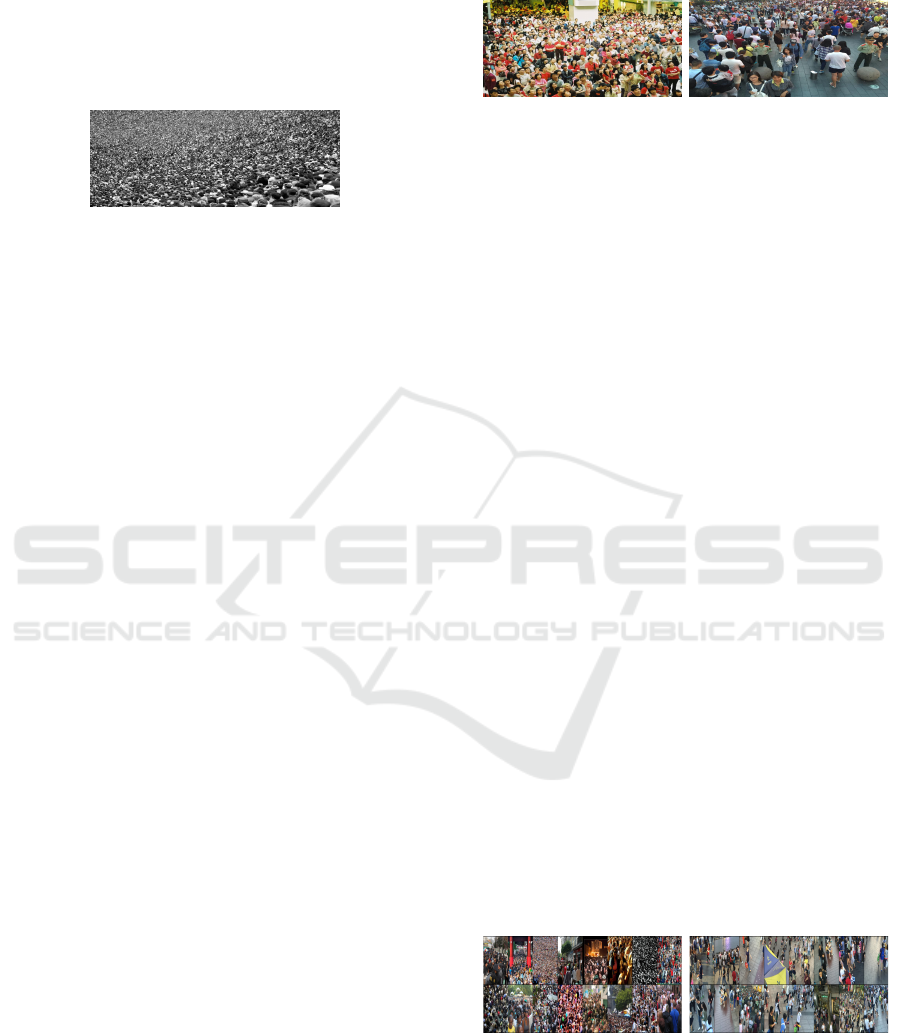
Figure 1: Example of an image from the UCF-CC-50. It is

possible to observe how the image presents people density

variation, with regions of extreme concentration.

Due to the scarcity in the amount of images, the

5-fold cross-validation strategy was employed, divid-

ing the original set into 5 groups, taking 4 groups for

training and 1 for testing, repeating the procedure for

each possible training and testing split. The results

presented comprise the average of the efﬁciencies in

each of the 5 folds, as well as the standard deviation.

4.1.1 Data Augmentation

Data augmentation processes were employed to ex-

pand the amount of data available for training in each

fold. The strategies aimed to reproduce the results ob-

tained by Quispe et al. (Quispe et al., 2020) and were

retained for later testing, allowing direct comparison

of models. Three forms of data augmentation were

adopted: (i) using a sliding window of 256×256 pix-

els, which scrolls through the images with a step of

70 pixels, cropping the new ﬁgures; (ii) adding Gaus-

sian noise (zero mean and variance 0.1) in half of

the images generated in the previous step and impul-

sive noise (with 4% probability of affecting a pixel) in

the other half, doubling the amount of samples; (iii)

changes in the illumination conditions (Equation 4)

of the images available after (ii), again doubling the

amount of images. The original images themselves

were not used.

′

(

+ 10, if i é even

1.25 f

− 50, otherwise

(4)

where f

′

is the output image and f

is the i-th image

available after step (ii).

4.2 ShanghaiTech

The ShanghaiTech database (Zhang et al., 2016) has

1198 images, split into two parts. The ﬁrst, Part A

contains 482 images obtained through the Internet,

separated into training and testing, while Part B is

composed of images obtained from streets of Shang-

hai (Figure 2).

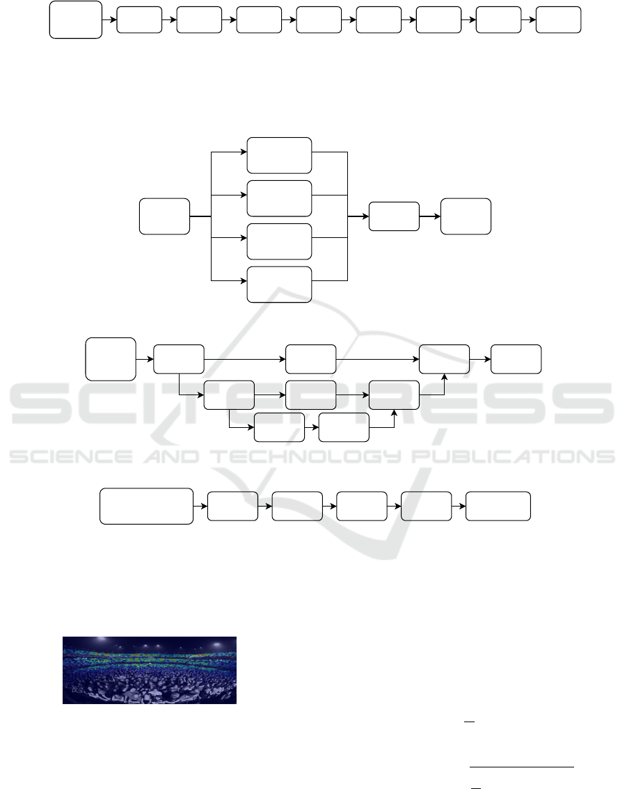
(a) Part A (b) Part B

Figure 2: Examples of images extracted from the two parts

of the ShanghaiTech database.

4.2.1 Data Augmentation

The procedures used to prepare the ShanghaiTech

images were different from those adopted for the

UCF-CC-50, in general, the process sought inspira-

tions from the original work of Zhang et al. (Zhang

et al., 2016), but adaptations were necessary to deal

with some constraints imposed by the proposed model

(Subsection 4.3). In short, the images must have

the dimensions of 256×256 pixels during the training

process, a condition that allows the mini-batch pro-

cessing and the use of the critical network.

The general idea of this data augmentation pro-

cess consists of making 5 cutouts of the original im-

age, one for each corner of the ﬁgure and a central

one, each cutout with the dimensions of 512×512. In

addition, for each one of the 5 new images, a horizon-

tal ﬂip was made, totaling 10 copies. Then, each of

the images was resized to 256×256 pixels, reaching

then the desired dimension for training.

There is a rare but actually occurring case at the

database, when an image has a height or width less

than 512 pixels, in which case the cropping process

would fail. To handle this case, images with height or

width less than 614 pixels – about 120% of 512 pixels

– were resized to have at least this amount of pixels

in their dimensions, but keeping the same proportion

of height and width, avoiding distortions. Once this

treatment was done, the procedure as described above

was applied normally. Some examples of the results

can be visualized in Figure 3.

(a) Part A (b) Part B

Figure 3: Examples of images extracted from the two parts

of the ShanghaiTech database after the data augmentation

process.

For the test images, it is not necessary to have the

dimensions of 256×256 pixels, so it was just resized,

Counting People in Crowds Using Multiple Column Neural Networks

365

halving the amount of pixels in height and width, in a

similar way to training.

4.3 Neural Network Architectures

The model used has two deep neural networks –

just as in a standard GAN model –, these being the

critical network (Figure 4) and a multi-channel neu-

ral network, which will be referred to as MCNN-U

(Figure 5), which is analogous to the generative net-

work of a Wasserstein-GAN, but whose input is a

monochromatic image rather than noise, as well as

using transposed convolutions to preserve the dimen-

sion of the density map and skip connections to in-

crease the complexity of the model, differentiating it

from previous (Quispe et al., 2020) models.

The MCNN employed is composed of 4 columns

– referred to as U-columns – of different ﬁlter sizes

(Figure 5). Each column consists of convolution and

max pooling operations that reduce the size of the ac-

tivation map, followed by transposed convolution op-

erations that recover the original map size (upscale).

In addition, skip connections have been added con-

necting the convolutional layers and the upscale lay-

ers, allowing the architecture to combine activations

from different depths of the network. It is worth men-

tioning that the 1×1 convolutions used in the skip

connections were employed with the purpose of re-

ducing the amount of transmitted channels, which

would make the model heavier, moreover, without

this reduction there would be more data from shallow

layers than deep layers.

4.4 Density Maps

The task of the MCNN-U is to produce a density map

whose summation corresponds to the amount of peo-

ple in the image. To produce the ground truth values,

given an image of dimensions M×N, a null matrix of

the same size is created. At the position of each per-

son, the value 1 is placed in the matrix, and ﬁnally, a

convolution is performed with a Gaussian ﬁlter (Fig-

ure 6), with dimensions 15×15, σ = 15.

4.5 Cost Function

The cost function used for training the described

neural networks can be divided into two parts, one

that corresponds to the basic goal of decreasing the

distance between the output of the MCNN-U – the

MCNN-U network will be denoted G, hence the out-

put of G for an image I is denoted G(I) – and the

ground truth value (gt); and another part that con-

cerns the Wasserstein cost of the adversarial network

model. The critical network will be denoted as C.

The distance between the density distribution

maps is given by the root mean square error of the

matrix values:

MSE

∑

i=1

∑

x=1

∑

y=1

[G(I

)(x, y) − gt(x, y)]

(5)

where M is the width and N is the height of the density

map, while m is the size of the batch.

On the other hand, the Wasserstein cost for the

generative network is given by:

= −

∑

i=1

C(G(I

)) (6)

Combining the two costs gives the cost of the gen-

erative network:

= L

MSE

+ αL

(7)

α being a hyperparameter to be decided.

The cost for the critical network is given by:

∑

i=1

C(gt

) −

∑

i=1

C(G(I

)) (8)

The method goal is to minimize the value of L

and maximize that of L

4.6 Test Conﬁguration

This subsection presents how the training and model

evaluation were conducted. Different versions of the

model with variations in hyperparameters were eval-

uated, but only the ﬁnal version will be presented in

this summary.

The Wasserstein cost was applied through the

value of α = 3,500 (Equation 7). In addition, the den-

sity maps were multiplied by 16,000. For each one

of the UCF-CC-50 training sets, 1,000 epochs were

run, with a batch size of 32 images. For ShaghaiTech,

Parts A and B, the value of 1,500 epochs was em-

ployed, with a batch size of 64 images.

The Rectiﬁed Adam (Liu et al., 2020) optimizer

was adopted, with learning rate lr = 1 · 10

−4

, β

0.9 and β

= 0.999. The value of ncritic, that is, the

number of times the critical network receives data and

is optimized for each pass through of the generative

network, was set to 3.

The algorithms were all executed using virtual

machines from Google Colaboratory. The machines

typically provide one core of an Intel Xeon (variable

model), about 12 GB of RAM and a graphics process-

ing unit (GPU) that can vary between an Nvidia Tesla

K80, an Nvidia Tesla P100 or an Nvidia Tesla T4.

VISAPP 2023 - 18th International Conference on Computer Vision Theory and Applications

366

Input Image

1x256x256

Conv

1,4,64

Input channels,

Filter size,

Output channels

Conv

64,4,64

Conv

64,4,128

Conv

128,4,256

Conv

256,4,512

Conv

512,4,512

Dimensions

Conv

512,4,1

Evaluation

Figure 4: Critical network architecture. The activation function used is the leaky ReLU (α = 0.02) and the convolutions have

parameters 4, 2 and 1 for the size of the kernel, stride and padding, respectively, the batch normalization technique is also

employed. The output layer has no activation function and the convolution has parameters 4, 1 and 0.

U-Column

MCNN-U

Fusion

Block

U-Column

K = 9

C = 12

U-Column

K = 7

C = 16

U-Column

K = 5

C = 20

U-Column

K = 3

C = 24

Input Image

1xMxN

Density Map

1xMxN

Dimensions

Input Image

1xMxN

Conv

C,K,2C

Conv

2C,K,C

Conv

C,K,C/2

Conv

C,K,C/4

Conv

1,(K+2),C

Pooling

Input channels,

Filter size,

Output channels

Upscale

Conv

2C,1,C/2

Conv

C/2,K,C/4

Upscale

Conv

C,1,C/4

Output

C/4xMxN

Concanated U-Column

outputs

18xMxN

Conv

18,1,18

Conv

18,3,9

Conv

9,3,4

Conv

4,3,1

Density Map

1xMxN

Fusion Block

Figure 5: MCNN-U Description. The tensor dimension is represented in the format <channels>×<width>×<height>, while

the convolutions, in the format <input channels>, <kernel size>, <output channels>, using an appropriate padding to maintain

the dimensions of the activation map; each convolution is followed by a ReLU activation function, except for the output layer.

The max pooling operation is used to halve the height and width dimensions, while upscale recovers the original dimension

with transposed convolutions with a kernel size = 2, stride = 2 and zero padding. 1×1 convolutions were used in the skip

connections to decrease the amount of transmitted channels.

Figure 6: Visualization of the density distribution map as a

heat map, overlaid with its original image, for the UCF-CC-

50 database.

4.7 Performance Metrics

To measure the performance (effectiveness) of the

tested networks, the sum of the density map of the

output of the generative network is compared with the

map generated through the Gaussian ﬁlter. To quan-

tify the difference between the two counts, two mea-

sures were employed:

• Mean absolute error:

MAE =

∑

i=1



cnt

− cnt

′



(9)

• Root mean square error:

RMSE =

∑

i=1

(cnt

− cnt

′

)

(10)

where N is the number of images in the test set, cnt

the correct count of people in image i, and cnt

′

is the

Counting People in Crowds Using Multiple Column Neural Networks

367

(a) Original image (b) Ground truth (c) MCNN-U (fold 2)

(d) Original image (e) Ground truth (f) MCNN-U fold 3)

Figure 7: Visualization of the density maps produced using the ground truth values and the MCNN-U for the UCF-CC-50

database.

Table 1: Efﬁciencies obtained by the MCNN-U model.

Metric Fold 1 Fold 2 Fold 3 Fold 4 Fold 5 Average Standard Deviation

MAE 424.5566 204.7662 197.8882 229.6904 225.2515 256.4306 84.9117

RMSE 709.0030 294.2144 323.6123 321.3106 345.6961 398.7673 155.9756

count made from the neural network output. Note that

these values only evaluate the count result and not the

content of the density distribution maps themselves.

For the UCF-CC-50 case in particular, the two

metrics are calculated for each of the 5 folds, and the

ﬁnal result is given by their average. The standard

deviation was also calculated, as it represents how

homogeneous the model’s effectiveness was for each

fold.

5 EXPERIMENTAL RESULTS

The ground truth density maps and those produced

by the MCNN-U for the same image can be viewed

by placing them side by side for comparison purposes

(Figure 7). In the upper ﬁgures, the network result

seems to match what was expected, but in the back-

ground, some regions of high density of people were

not identiﬁed – which can also be conﬁrmed in Fig-

ure 8. In the lower images, a more critical case is

presented, with a large number of false positives in

the tree leaf region.

Table 2: Comparison of the effectiveness achieved by the

MCNN-U in the UCF-CC-50 database in relation to other

models in the literature.

Model

Mean Mean

MAE RMSE

MCNN (Zhang et al., 2016) 377.6 509.1

MSNN

(Quispe et al., 2020) 374.0 554.6

CP-CNN (Sindagi and Patel, 2017) 295.8 320.9

MCNN-U 256.4 398.8

CAN (Liu et al., 2019) 212.2 243.7

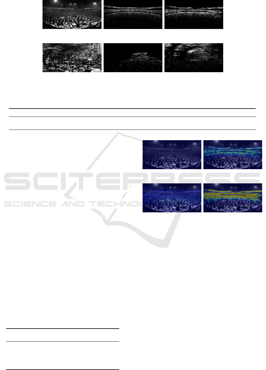
(a) Column 0 (b) Column 1

Figure 8: Visualization of the activation maps for each of

the columns of the MCNN-U in the UCF-CC-50 database,

column 0 (a) being the one with the largest ﬁlter size, and

column 3 (d) being the smallest. A Gaussian ﬁlter was ap-

plied to the LayerCAM output to improve the map visual-

ization.

Using the LayerCAM described previously, it is

possible to independently observe the behavior of

each column of the MCNN-U (Figure 8). It is notice-

able that each column was more (or less) activated

in different regions of the image, due to the varia-

tion in density of people, column 0 was not activated,

while column 1 and especially column 3 focused on

the region of higher density, while column 2 identi-

ﬁed the larger people, with emphasis on the region

of the heads. The results obtained after training the

MCNN-U on the UCF-CC-50 database, for the hyper-

parameters deﬁned in Subsection 4.6 were compiled

in Table 1, separated by fold.

The effectiveness of the model was relatively con-

stant across all but the ﬁrst fold. This pattern was

VISAPP 2023 - 18th International Conference on Computer Vision Theory and Applications

368

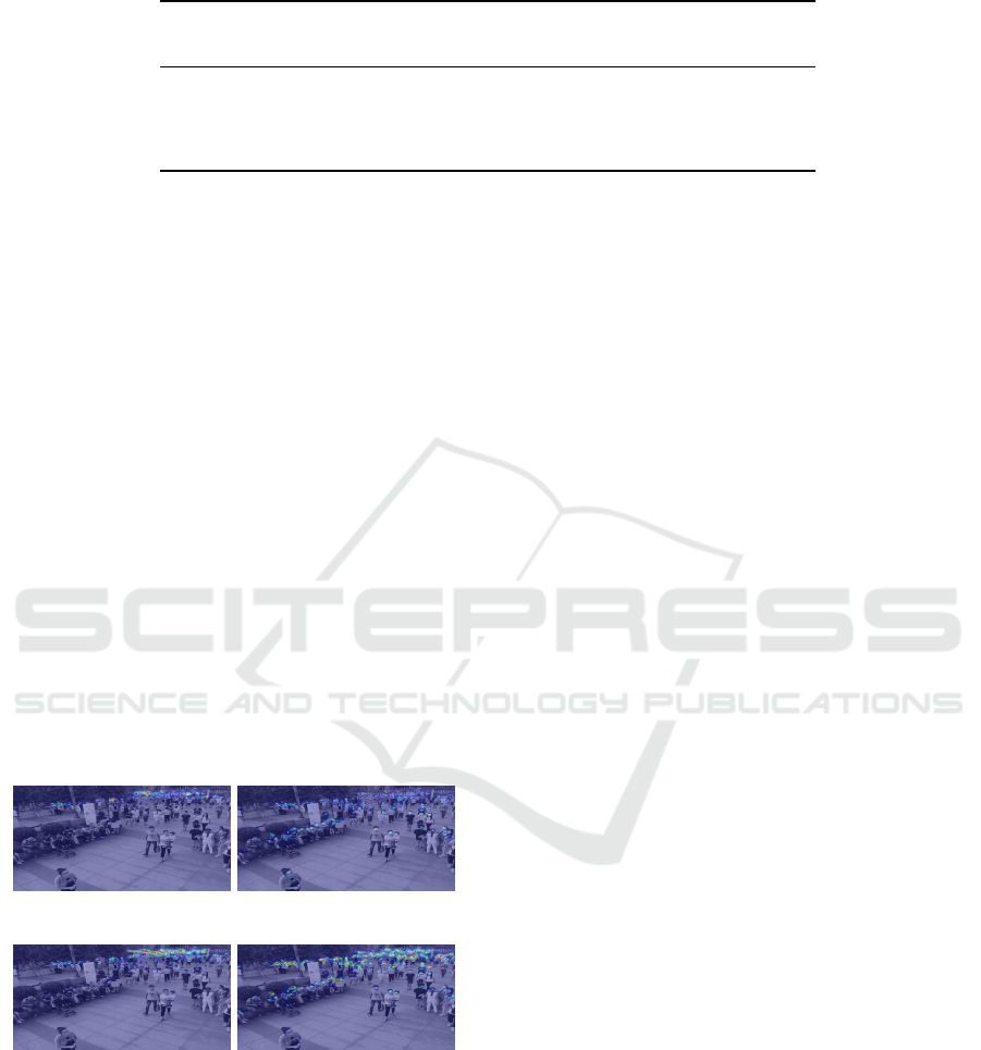
Table 3: Comparison of the effectiveness achieved by the MCNN-U in the ShanghaiTech database in relation to other models

in the literature.

Model

Part A Part B

Mean Mean Mean Mean

MAE RMSE MAE RMSE

MSNN

(Quispe et al., 2020) 163.4 242.7 34.5 57.7

MCNN (Zhang et al., 2016) 110.2 173.2 26.4 41.3

MCNN-U 105.5 152.4 18.3 30.0

CP-CNN (Sindagi and Patel, 2017) 73.6 106.4 20.1 30.1

CAN (Liu et al., 2019) 62.3 100.0 7.8 12.2

repeated throughout previous model tests, this being

the most challenging partition of the database, possi-

bly due to the high density of the test images. In order

to be able to evaluate the effectiveness achieved by

MCNN-U, the performance metrics were compared

with other results from the literature (Table 2).

The efﬁciency obtained represents a leap when

compared to the original MCNN, demonstrating that

the modiﬁcations applied were indeed appropriate to

the model. In relation to the approaches of the lit-

erature, the results were competitive, but more com-

plex approaches that seek to evaluate the image con-

text obtained higher efﬁciencies, which may, on the

other hand, result in more complex training.

For the ShanghaiTech database, on the other hand,

Part A has images with people densities comparable

to the UCF-CC-50 database, while Part B, despite

having photos of busy streets, the people counts are

generally lower, with considerable portions of the im-

ages without people. It is especially interesting to ob-

serve the behavior of the MCNN-U for these cases of

less dense images (Figure 9).

(a) Column 0 (b) Column 1

Figure 9: Visualization of the activation maps for each

one of the MCNN-U columns in the ShanghaiTech Part B

database, column 0 (a) being the largest ﬁlter size, and col-

umn 3 (d) being the smallest. A Gaussian ﬁlter was applied

to the LayerCAM output to improve the visualization of the

map.

It can be seen in this case that, unlike the acti-

vations for UCF-CC-50, here all columns were acti-

vated for some part of the image, while in Figure 8,

the column with the largest ﬁlter was not activated.

One concern that existed was that many false pos-

itives would occur in the empty regions of the im-

age, but looking at this result and others, this does not

seem to be the case. Still on Part B, training on this

database was considerably more unstable than Part A,

or any other fold of the UCF-CC-50, with the cost

function showing sudden spikes during training (Ta-

ble 3). Whether this was caused by a numerical insta-

bility of the RAdam optimizer or whether it is an in-

trinsic characteristic of the model combined with the

database, deﬁning a space with many local minima, is

still an uncertain aspect, further tests with other con-

ﬁgurations of the optimizer are needed.

Unlike what was observed with the UCF-CC-50

tests, the increase in efﬁciency obtained with the

MCNN-U when compared to the MCNN model was

considerably lower, especially in Part A. A possible

reason for this difference lies in the data augmenta-

tion process. In fact, the model of Zhang et al. was

trained under different conditions, the data treatment

was not the same, as well as the training process. The

main difference would be in the fact that the MCNN

was trained one image at a time, without mini-batch,

and this allows the training images to have different

dimensions, for example. Other factors such as opti-

mizer settings may also affect, and the fact that Part

B training was more unstable, as mentioned earlier,

may point in the direction that the data augmenta-

tion process or the ShanghaiTech training guidelines

themselves need more adjustment for MCNN-U.

6 CONCLUSIONS

The effectiveness obtained by the MCNN-U was con-

siderably higher compared to the original MCNN in

the best case scenario. The proposed changes to the

model were tested incrementally and the experiments

with ShanghaiTech Part B indicated that there is room

for improvement in the model in terms of stability,

possibly with further testing on other optimizers or

by adding modiﬁcations to the network to achieve

smoother convergence.

Counting People in Crowds Using Multiple Column Neural Networks

369

REFERENCES

Arjovsky, M., Chintala, S., and Bottou, L. (2017). Wasser-

stein Generative Adversarial Networks. In Precup, D.

and Teh, Y. W., editors, 34th International Confer-

ence on Machine Learning, volume 70, pages 214–

223. PMLR.

Gao, G., Gao, J., Liu, Q., Wang, Q., and Wang, Y. (2020).

CNN-based Density Estimation and Crowd Counting:

A Survey. arXiv preprint arXiv:2003.12783, pages 1–

25.

Idrees, H., Saleemi, I., Seibert, C., and Shah, M.

(2013). Multi-source Multi-scale Counting in Ex-

tremely Dense Crowd Images. In IEEE Conference

on Computer Vision and Pattern Recognition, pages

2547–2554.

Jiang, P.-T., Zhang, C.-B., Hou, Q., Cheng, M.-M., and Wei,

Y. (2021). LayerCAM: Exploring Hierarchical Class

Activation Maps for Localization. IEEE Transactions

on Image Processing, 30:5875–5888.

Lempitsky, V. and Zisserman, A. (2010). Learning to Count

Objects in Images. Advances in Neural Information

Processing Systems, 23:1324–1332.

Li, M., Zhang, Z., Huang, K., and Tan, T. (2008). Estimat-

ing the Number of People in Crowded Scenes by Mid

based Foreground Segmentation and Head-shoulder

Detection. In 19th International Conference on Pat-

tern Recognition, pages 1–4. IEEE.

Liu, L., Jiang, H., He, P., Chen, W., Liu, X., Gao, J.,

and Han, J. (2020). On the Variance of the Adaptive

Learning Rate and Beyond. In Eighth International

Conference on Learning Representations, pages 1–14.

Liu, W., Salzmann, M., and Fua, P. (2019). Context-Aware

Crowd Counting. In IEEE Conference on Computer

Vision and Pattern Recognition, pages 5099–5108.

Quispe, R., Ttito, D., Rivera, A., and Pedrini, H. (2020).

Multi-Stream Networks and Ground Truth Generation

for Crowd Counting. International Journal of Electri-

cal and Computer Engineering Systems, 11(1):33–41.

Selvaraju, R. R., Cogswell, M., Das, A., Vedantam, R.,

Parikh, D., and Batra, D. (2017). Grad-CAM: Vi-

sual Explanations From Deep Networks via Gradient-

Based Localization. In IEEE International Confer-

ence on Computer Vision, pages 618–626.

Sindagi, V. A. and Patel, V. M. (2017). Generating High-

Quality Crowd Density Maps Using Contextual Pyra-

mid CNNs. In IEEE International Conference on

Computer Vision, pages 1879–1888.

Zhang, Y., Zhou, D., Chen, S., Gao, S., and Ma, Y. (2016).

Single-image Crowd Counting via Multi-column Con-

volutional Neural Network. In IEEE Conference on

Computer Vision and Pattern Recognition, pages 589–

597.

VISAPP 2023 - 18th International Conference on Computer Vision Theory and Applications

370