Fast Heuristic for Ricochet Robots

Jan H

ula

1,2 a

, David Adamczyk

1 b

and Mikol

s Janota

2 c

Institute for Research and Applications of Fuzzy Modeling, University of Ostrava,

Ostrava, 701 03, Czech Republic

Czech Technical University in Prague, Prague, Czech Republic

Keywords:

Multi-Agent Pathﬁnding, Heuristic Algorithms, Ricochet Robots, Subgoals.

Abstract:

In this contribution, we describe a fast heuristic for a logical game called Ricochet Robots in which multiple

robots cooperate in order to reach a goal. The heuristic recursively explores a restricted search space using

subgoals that correspond to interactions of two robots. Subgoals are expanded according to an estimated length

of a complete solution, which makes the algorithm reminiscent of the A* algorithm. The estimated length is

a lower bound of the length of the real solution, and this allows us to prune subgoals using the best solution

found thus far. After eliminating all remaining subgoals, we are guaranteed that the best solution found is the

shortest solution from the restricted search space. Moreover, we show that the restricted search space contains

a large portion of optimal solutions of the empirical distribution of 1 million random problems. We believe that

the presented ideas should generalize to other search problems in which multiple independent agents could

block or help each other.

1 INTRODUCTION

This contribution presents a fast heuristic (Edelkamp

and Schrodl, 2011; Pearl, 1984) for a logical game

called Ricochet Robots. In this game, the player con-

trols independent robots placed on a grid with obsta-

cles and tries to get one particular robot to the desired

goal position, ideally in the least amount of steps. The

heuristic is based on several novel ideas which should

generalize to other search problems in which multi-

ple independent agents could block or help each other.

The main idea stems from the fact that empirically the

distribution of randomly generated problems induces

optimal solutions with a property that we can exploit

to restrict the search space.

Our approach works by enumerating all possible

solutions with this property. The search can be viewed

as a version of the A* algorithm (Hart et al., 1968)

that searches over the state space of possible meeting

points of pairs of robots. Two types of relaxations for

the length of a path are used to effectively prune the

search space.

The text of this contribution is structured as fol-

lows: In Section 2 we describe the problem, in Sec-

https://orcid.org/0000-0001-7639-864X

https://orcid.org/0000-0002-7794-104X

https://orcid.org/0000-0003-3487-784X

tion 3 we present an empirical distribution of optimal

solution types which serves as a motivation for our

approach, in Section 4, the search algorithm is de-

scribed, Section 5 contains experimental results, Sec-

tion 6 contains related work which is followed by dis-

cussion and conclusion in Sections 7 and 8, respec-

tively.

2 PROBLEM DESCRIPTION

Ricochet Robots is a puzzle board game designed by

A. Randolph. The player controls multiple movable

pieces (robots) placed on a square grid with several

obstacles (walls) between two adjacent tiles. The

robots are allowed to move only in vertical or hori-

zontal directions and once they start moving, they can

stop only when blocked by a wall or another robot.

The goal is to cover target tiles with robots of the cor-

responding color with the least number of moves. In

our case, we will focus on games with only one target

tile.

Each step of a game consists of selecting a robot

and a direction. Before executing the next move, the

previous move needs to be fully executed. To reach

the target tile, the corresponding robot may need the

assistance of other robots to stop at tiles from which

H˚ula, J., Adamczyk, D. and Janota, M.

Fast Heuristic for Ricochet Robots.

DOI: 10.5220/0011699900003393

In Proceedings of the 15th International Conference on Agents and Artiﬁcial Intelligence (ICAART 2023) - Volume 1, pages 71-79

ISBN: 978-989-758-623-1; ISSN: 2184-433X

 2023 by SCITEPRESS – Science and Technology Publications, Lda. Under CC license (CC BY-NC-ND 4.0)

it can get to the target tile. The helper robots may

also need assistance from other robots, and this makes

the reachability problem interesting. The game with

k robots and one target tile was proven to be NP-

Complete by Engels et al. (Engels and Kamphans,

2006). For completeness, we provide a formal def-

inition of the game adapted from Masseport et al.

(Masseport et al., 2019):

Deﬁnition 1. Ricochet Robots is a class of 1-player

games parametrized by the size of a grid and the num-

ber of robots. The board state of this game with grid

size n × n and k robots consists of:

1. A square grid of size n × n

2. A set R = {r

,...,r

} of k robots where r

= (x

)

with 1 ≤ x

≤ n. The robot r

is designated to

be the target robot.

3. A target tile g = (x

)

4. A set O = {{(o

),(o

)} : |o

− o

| + |o

−

| = 1} of obstacles with 1 ≤ o

≤ n

A game state is valid if ∀i(¬∃ j((i 6= j) ∧ (r

))). In plain language, two robots cannot be in the

same position at the same time. The goal of the game

is to reach a state where r

= g. Possibly, we may

rank solutions by the number of moves they contain.

The rules of the game could be described

as follows: At each move, the player se-

lects a robot r

= (x

) and a direction d ∈

{(0,1),(0,−1),(1,0),(−1,0)}. The board state is

updated by deleting the robot at position (x

) and

adding it at position (x

) + dt, where t is the small-

est value such that (x

) + dt + d ∈ R or {(x

) +

dt,(x

) + dt + d} ∈ O. In plain language, the robot

moves in the chosen direction until it is blocked by

another robot or by an obstacle.

In order to make the problem easily visually un-

derstood, the individual robots are colored and the tar-

get tile has the same color as the target robot.

3 EMPIRICAL DISTRIBUTION

OF SOLUTION TYPES

The heuristic we use to ﬁnd the solution can be justi-

ﬁed by the fact that, empirically, the optimal solutions

(with the least number of moves) tend to have the

property which we call Simple Reverse Dependency

(SRD). Concretely, this property holds for ∼ 94% of

1 million randomly generated instances. In this sec-

tion, we describe how we computed this number.

Generating Data for the Analysis. First, we gener-

ated 1 million random instances as described in Sec-

tion 5.1. In this case, we generated instances of size

16 × 16. For each instance, we ﬁnd the shortest so-

lution with a publicly available solver designed and

optimized for Ricochet Robots

with a runtime of 60

seconds. Given an optimal solution, we need to ex-

plain every move in it. The purpose of every move

can be to avoid or help another robot, with the excep-

tion that the target robot can also move to reach the

target tile. There could also be moves whose purpose

is to avoid some robot and help another robot at the

same time. We count the moves as helping moves.

To label each move, we iterate over all the moves

of a given robot until a state in which this robot is

helping another robot (the other robot is blocked by

it). If there is such a state, we label all the pre-

vious moves as helping moves, and the subsequent

moves as still unexplained. If there is no such state,

we label all the moves either as avoidance moves or

target-reaching moves, depending on whether they are

done by a helper robot or a target robot, respectively.

We follow this procedure until all the moves of every

robot are explained.

Solution Dependency Graph. Next, we construct

a Solution Dependency Graph. This is a multigraph

(parallel edges are allowed) where the nodes corre-

spond to individual robots and the edges correspond

to sequences of moves. The edges are labeled by the

purpose of the moves. For example, if there is a se-

quence of moves of a green robot whose purpose is

to stop the red robot on a given tile, there will be an

edge from the node of the green robot to the node of

the red robot labeled by the type of interaction help. If

the green robot is avoiding the red robot, there would

be the same edge labeled by type of interaction avoid-

ance.

In order to deﬁne and detect the SRD property, we

also need to assign an index to the incoming edges of

the interaction type help. This index reﬂects the tem-

poral order of helping interactions. This means that if

two robots are helping another robot, we will be able

to read out of the graph which helping interaction was

realized ﬁrst

. The indexing is done independently for

each node (i.e. for every set of edges incoming to that

node of interaction type help).

Representing the optimal solution as such a graph

enables us to count how many times a solution of each

type occurs in the sample of the million random in-

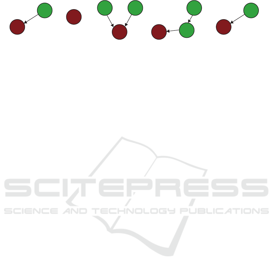
stances. In Figure 1, we show the ﬁve types of the

most frequent solutions together with a percentage of

solutions covered by each solution type. We can also

https://github.com/fogleman/Ricochet

The helping interaction is realized once the helped

robot stops by being blocked by the helping robot.

ICAART 2023 - 15th International Conference on Agents and Artiﬁcial Intelligence

~33% ~7% ~6% ~4%~35%

help 1

help 1 help 2

avoid

help 1

Figure 1: Five most frequent solution types. Nodes with T represent target robots, nodes with H represent helper robots. To-

gether, these types of solutions cover ∼ 85% of 1 million randomly generated solutions. The index of the edges of interaction

type help reﬂects the temporal order as mentioned in the main text.

count the number of solutions with the SRD property,

which is deﬁned next.

Simple Reverse Dependency Property. We say

that a Solution Dependency Graph has a Simple Re-

verse Dependency property if the following condi-

tions hold:

1. The multigraph is a tree.

2. There is no node in the graph that would have an

incoming and outgoing edge of interaction type

help and where the outgoing edge would have an

index strictly greater than 1.

These conditions specify the property of all solu-

tions, which can be found by our algorithm.

We found that from the sample of 1 million in-

stances, ∼ 94% of the solutions have this property.

This ﬁnding justiﬁes the use of our heuristic, which

effectively searches for the shortest solutions with this

property. We call the space of solutions with this

property a restricted search space. We note that if

the actual shortest solution of the game does not have

this property, then there is still a high chance that a

longer solution with this property will exist, and our

method will ﬁnd it.

4 THE APPROACH

4.1 High-Level Overview

On a high level, our algorithm recursively searches

over subgoals between the current and the goal state.

At each level of the recursion, the expanded sub-

goal becomes a current goal, and new subgoals are

proposed. These could be expanded further until a

feasible solution is found. The subgoals are being

expanded according to their optimistically estimated

cost, which serves as a lower bound of the real cost

(length of the ﬁnal solution). This makes the algo-

rithm reminiscent of the A

search, but here we search

over subgoals instead of the low-level states. If a

feasible solution is found at some point, its real cost

can be used to prune the search space by removing

subgoals whose lower bound is higher than the cost

of this feasible solution. This pruning enables us to

quickly search over all possible subgoals until no un-

explored subgoal remains, and this, in turn, guaran-

tees that we will ﬁnd the shortest solution of the re-

stricted search space.

In the following sections, we describe the whole

approach in detail. Section 4.2 describes how the sub-

goals are enumerated at each node of the recursion

tree. Section 4.3 describes the estimation of the cost

of the ﬁnal solution corresponding to a subgoal and ﬁ-

nally, Section 4.4 contains a pseudocode of the search

algorithm.

4.2 Enumeration of all Possible

Subgoals Between the Current and

the Goal State

Starting from the initial state of the game where the

goal is to cover the target tile with the target robot,

our algorithm recursively creates subgoals, which are

states that should be traversed in the ﬁnal solution.

Each subgoal in the current level of recursion corre-

sponds to a state in which one robot is helping the cur-

rent target robot to stop at a position from which it can

reach the current goal state without any other help. In

order to reach such a state, the helper robot needs to

reach its helping position, and the target robot needs

to reach the position where the helper robot blocks it.

To efﬁciently enumerate the subgoals, we consider

only such states where either the target robot or the

helper robot can reach their position in the subgoal

state without any further help. For example, if we

know that the helper robot is able to reach its helping

position in the subgoal then the subgoal will be com-

pleted if we ﬁgure out how to move the target robot to

its corresponding position in this subgoal.

When we expand the subgoal during the search,

the position of the robot with unknown reachability

status becomes a goal and the whole procedure is

Fast Heuristic for Ricochet Robots

repeated. At every node of the recursion tree, the

only robots that can be used as helpers are only the

ones that have still not been used on the path from

the root of the recursion tree to this node. This

means that every robot will be able to help only once.

To quickly obtain possible subgoals for the target or

helper robots, we use the following data structure.

The Graph of Components. Each layout of the

game can be represented as a directed graph where

nodes correspond to tiles and edges to possible tran-

sitions between two tiles. That is, there is a directed

edge between two nodes if the robot can transition

from the source tile to the target tile in one move.

A natural concept in such a graph is a strongly con-

nected component. It consists of a maximal collec-

tion of nodes so that it is possible to reach every node

within the component from every other node within

the component. The graph of the typical grid will

consist of several such components as depicted in Fig-

ure 2.

As visible in this Figure 2 (graph a)), the compo-

nents could be related by reachability, and therefore

we can construct a new graph of components where

there is an edge from component a to component b,

if it is possible to transition from component a to

component b. This graph, which we call reachability

graph, allows us to efﬁciently query all the compo-

nents reachable from a given tile. We simply check

the components which contain the tile and then return

them together with all their descendants in this graph.

For a tile x, we denote this set of components by ↓(x).

The same can be done to obtain the set ↑ (x) of all

components from which it is possible to reach the tile

x, with the only difference being that we take all an-

cestors. For small grids, these two mappings from

tiles to components can be cached in a dictionary.

If it is possible to reach tile b from tile a without

any help, then ↓ (a)∩ ↑ (b) 6=

0. If there is the possi-

bility to reach the tile b from the tile a with exactly

one help from another robot, then the robot that starts

at the tile a will at some point need to transition from

one of the components of ↓ (a) to one of the compo-

nents of ↑(b). This transition will be done by a move

in which the starting tile is still in ↓ (a) but the end

tile is already in ↑ (b). We call the starting tile a pre-

transition tile and the end tile a transition tile. In this

move, the moving robot needs to be blocked by an-

other helping robot that is adjacent to the transition

tile. We call this tile a supporting tile.

Subgoals for the Helper Robots. Therefore, to

enumerate all subgoals that allow the target robot to

reach a tile b from a tile a, we need to ﬁnd all tiles

that allow the robot to transition from ↓ (a) to ↑ (b).

For that end, we construct another graph, we call tran-

sition graph for the target robot, with the nodes again

corresponding to components and edges correspond-

ing to possible transitions from one component to the

other. In comparison to the ﬁrst graph, the edges go

in the opposite direction, and we ignore the edges cor-

responding to transitions that are possible without the

assistance of another robot. For the grid in Figure 2,

there would be an edge that goes from the green com-

ponent to the red component but not the edge that goes

in the opposite direction. If there are multiple tiles

that allow for the transition from one component to

the other, we add edges for all of them as visible in

Figure 2 b).

These edges will represent subgoals that could be

satisﬁed by the helper robots. For example, if there is

an edge going from ↓(a) to ↑(b) and ↓(a)∩ ↑(b) =

we know that there is a pretransition tile in one of

the components of ↓(a) reachable from a and we also

know that there is a transition tile in one of the com-

ponents of ↑ (b) from which it is possible to reach b.

Therefore, the only thing we do not know is whether

some helper robot is able to reach the corresponding

supporting tile, and this creates a candidate for a new

subgoal.

Subgoals for the Target Robot. We also need to

take into consideration subgoals for the target robot

for which we know that some helper robot is able to

reach the supporting tile but do not know whether the

target robot is able to reach the pretransition tile. To

enumerate such subgoals for the target robot, we cre-

ate a third graph, we call transition graph for helper

robots, with edges that go from components contain-

ing the supporting tile to components containing the

transition tile. For the grid in Figure 2, we would add

an edge from the blue to the red component because a

robot in the blue component could help a target robot

to get to the red component. The resulting graph is

visible in Figure 2 c).

With each edge, we also store additional informa-

tion to fully specify the subgoal. These include the

positions of the transition, pretransition, and support-

ing tiles. For every transition tile, there are two possi-

ble pairs of the pretransition and supporting tiles be-

cause the moving robot can approach the transition

tile from one of the two directions and the support-

ing tile must be adjacent to the transition tile on the

opposite side as depicted in Figure 3. In the transi-

tion graph for the target robot, we therefore need to

store these two pairs of tiles for every edge or create

two separate edges, which is what we do in our im-

plementation.

ICAART 2023 - 15th International Conference on Agents and Artiﬁcial Intelligence

b) c)

green

red

blue

yellow

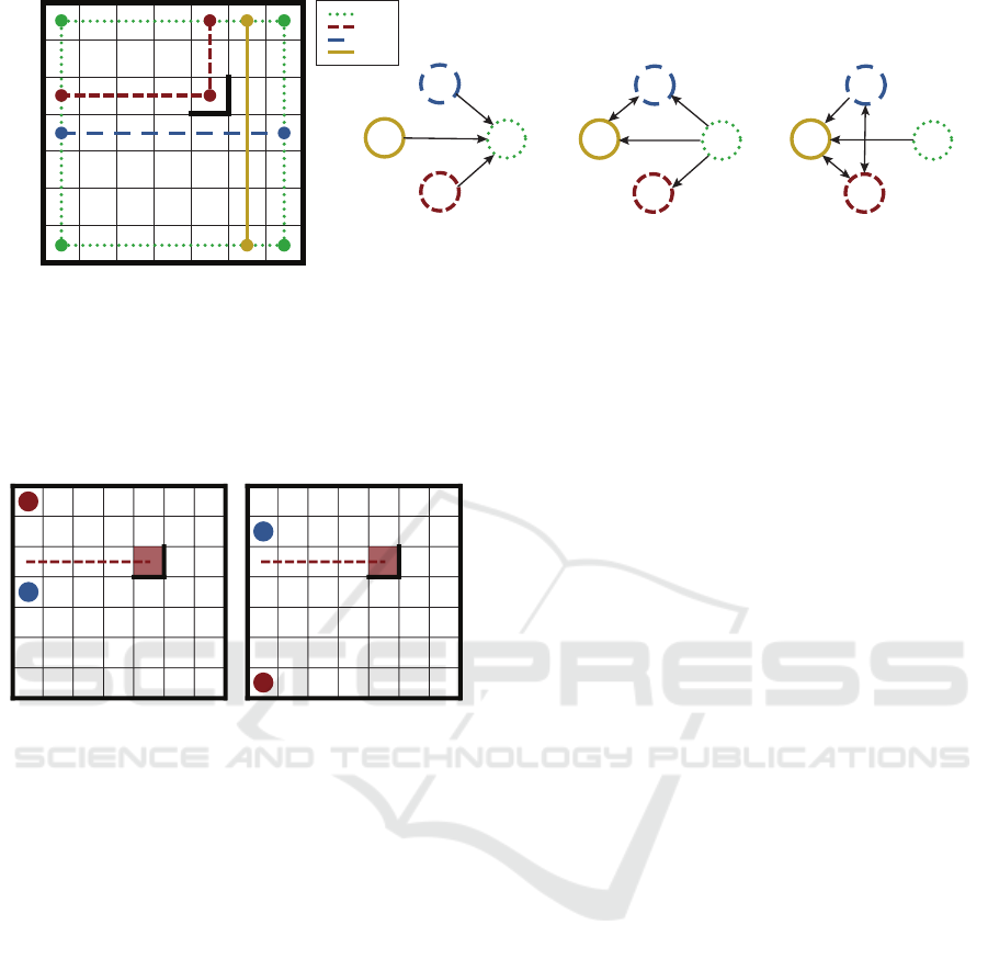
Figure 2: Component and transition graphs. The grid on the left shows four components of the grid with the nodes of

each component highlighted by a dot. Note that there are other components corresponding to vertical and horizontal lines

which are not shown here. The 3 different relations between these components are depicted in the graphs on the right. a) The

graph of connected components shows which components are reachable from a given component without any assistance. b)

The transition graph for the target robot shows which components are reachable from a given component with exactly one

assistance. c) The transition graph for helper robots shows which components could be used in order to assist some robot to

reach the desired component. For example, the arrow from the green to the yellow node reﬂects the fact that some position in

the green component (i.e., the top-right corner) can be used to assist some other robot to transition to the yellow component.

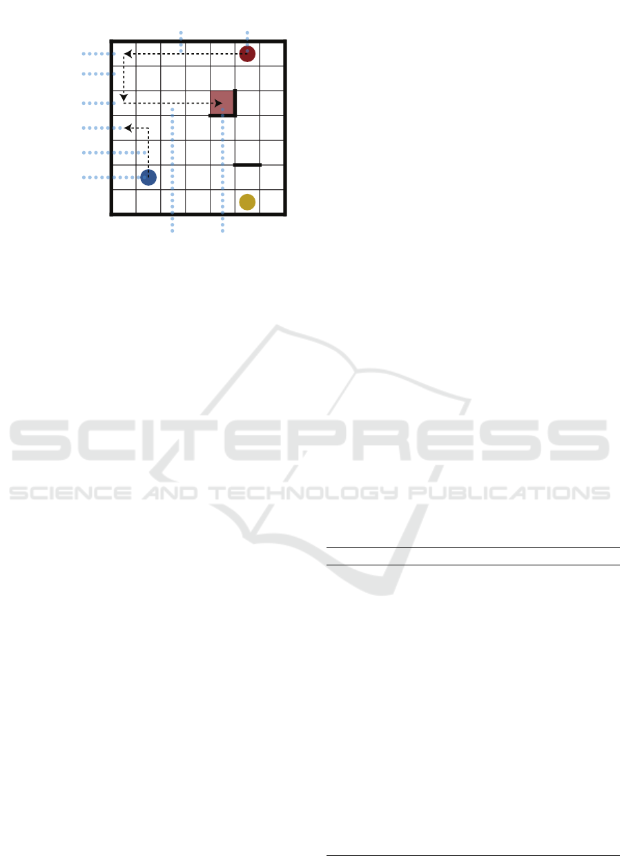
Figure 3: This ﬁgure shows that for the transition tile at po-

sition (3, 1) that enables the red robot to transition to the red

component, there are two pairs of pretransition and support-

ing tiles. This holds in general, for every transition tile there

are two such pairs.

In order to enumerate all helper subgoals which

help the target robot to get from the tile a to the tile b,

we do the following steps:

4.2.1 Obtaining all Subgoals for the Available

Helper Robots

1. obtain ↓(a) and ↑(b) from the reachability graph.

2. get all edges in the transition graph for the target

robot that go from ↓(a) to ↑(b).

3. for each edge and each available robot at the cur-

rent recursion level, create a new subgoal in which

the helper robot needs to reach the supporting tile

stored in the edge.

4. with each new subgoal, store a reference to a par-

ent subgoal together with the transition and pre-

transition tiles so that we can later reconstruct

the path.

In order to enumerate all target subgoals where

the helper robot at tile c helps the current target robot

reach the tile b, we do the following steps:

Obtaining all Subgoals for the Current Target

Robot.

1. obtain ↓ (c) and ↑(b) from the reachability graph.

2. get all the edges in the transition graph for helper

robots that go from ↓(c) to ↑(b).

3. for each edge and the current target robot, create

a new subgoal in which the target robot needs to

reach the pretransition tile stored in the edge.

4. with each new subgoal, store a reference to a par-

ent subgoal together with the transition and sup-

porting tiles so that we can later reconstruct the

path. At the ﬁrst level of recursion, the parent sub-

goal is the original goal.

These four steps will be executed for all the available

robots at the current recursion level.

4.3 Estimating the Cost of Subgoals

As mentioned in Section 4.1, we may estimate the

cost of each subgoal and then expand the subgoals

from the most promising to the least promising. By

estimating the cost, we mean that we estimate the

length of the full solution of the game which factor-

izes through this subgoal. Each subgoal has a known

and an unknown component. The cost of the subgoal

s has the following form:

f (s) = g(s) +h(s) (1)

where g is the estimated cost of the known component

and h is the estimated cost of the unknown compo-

nent.

Fast Heuristic for Ricochet Robots

s.p

min

(s.a,s.p)

min

(s.c,s.s)

min

(s.t,s.b)

s.a

s.t

s.s

s.b

s.c

Figure 4: Illustration of individual terms used to compute

the estimate cost f (s) of a subgoal s shown in Equation 1.

To explain how these costs are estimated for both

the target and helper subgoals, we ﬁrst introduce the

following variables. The value of each variable is

given by the context of the subgoal:

• s.a — the position of the target robot

• s.b — the position of the target tile

• s.c — the position of the helper robot

• s.t — the position of the transition tile

• s.p — the position of the pretransition tile

• s.s — the position of the supporting tile

• s.parent — the reference to the parent subgoal

We also introduce the following distance mea-

sures:

• d

min

(x,y) — the length of the shortest path from

tile x to tile y on a grid with no robots

•

min

(x,y) — the length of the shortest path from

tile x to tile y on a grid with no robots and relaxed

rules of the game which allow the robot to stop at

every tile during the move

Both distance measures are relaxations. The ﬁrst one

ignores the robots that could potentially block the

path and may need to move in order to avoid the mov-

ing robot. The second one is much looser relaxation,

because it will always give a lower value than the ﬁrst

one. If the tile y is unreachable from the tile x with-

out the help of other robots, the ﬁrst measure will re-

turn ∞, but the second will return a lower bound of

the cost of the solution using other robots. Both of

these distance measures could easily be precomputed

for each pair of tiles using the Floyd–Warshall algo-

rithm (Floyd, 1962).

The Estimated Cost for the Helper Robot Sub-

goals. In order to estimate the cost f (s) of the sub-

goal of a helper robot, we use the following expres-

sions for g and h:

g(s) = d

min

(s.a,s.p)+d

min

(s.t, s.b)+1+g(s.parrent)

h(s) =

min

(s.c,s.s)

The +1 is for the move from the pretransition tile s.p

to the transition tile s.t and g(s.parent) is the cost we

accumulated with the subgoals of the ancestor. The

cost of the unknown component h is given by relax-

ation, which allows the robot to stop at any given tile

during the move. In Figure 4, we highlight the indi-

vidual terms in this cost.

The Estimated Cost for the Target Robot Subgoals.

For the subgoals of the target robot we have:

g(s) = d

min

(s.c,s.s) +d

min

(s.t, s.b) + 1 + g(s.parent)

h(s) =

min

(s.a,s.p)

Here, the expressions are similar to the ﬁrst case, but

we swap the roles of the target and helper robots.

4.4 Obtaining the Shortest Solution of

the Restricted Search Space

After deﬁning the enumeration of subgoals and es-

timation of their cost, we now describe the overall

algorithm which ﬁnds the shortest solution of the re-

stricted search space for the given instance. The pseu-

docode is visible in Algorithm 1.

Algorithm 1: Search for the shortest solution.

Input: instance of the game I

Output: shortest solution from the restricted search

space

1: info = preprocess(I)

2: ﬁnalGoal = info.goal

3: frontier = PriorityQueue()

4: frontier.put(ﬁnalGoal)

5: incumb = None

6: while len(frontier) 6= 0 do

7: current = frontier.get()

8: subgoals = getSubgoals(current,info)

9: subgoals = evaluate(subgoals)

10: incumb = getIncumb(subgoals,incumb,info)

11: frontier.merge(subgoals)

12: frontier = pruneSubgoals(frontier,incumb)

13: end while

14: return incumb

ICAART 2023 - 15th International Conference on Agents and Artiﬁcial Intelligence

The whole algorithm resembles A

search which

uses a priority queue to always expand the node with

the lowest estimated cost. In our case, the queue pri-

oritizes subgoals according to the estimated cost com-

puted by f from Equation 1.

The function preprocess precomputes the com-

ponent graphs mentioned in Section 4.2, the re-

laxed distance measures mentioned at the end of Sec-

tion 4.3, and extracts the speciﬁcation of the ﬁnal

goal. The function getsSubgoals generates the sub-

goals for the target and the helper robots as was de-

scribed in Section 4.2. The function evaluate eval-

uates the subgoals as described in Section 4.3. The

function getIncumb checks if any of the current sub-

goals are reachable without further assistance and re-

turns the solution as a current incumbent if its cost

is lower than the cost of the old incumbent. Other-

wise, it returns the old incumbent. Lastly, the function

pruneSubgoals iterates over all subgoals expanded

so far and removes them if their estimated cost (which

acts as a lower bound) is higher than the cost of the

current incumbent solution. During the search, this

pruning eliminates many potential subgoals and en-

ables us to completely explore the restricted search

space in a short time. Finally, we return the solution

with the least number of moves.

There is one detail that we omitted here. The func-

tion getIncumb needs to internally check if a given

subgoal could be realized without further assistance.

For this, it is necessary that the target robot of this

subgoal is able to reach the target tile of this subgoal.

Nevertheless, this is not sufﬁcient. The solution rep-

resented by the realizable subgoal was constructed by

considering paths on an empty grid (whose length was

estimated by the distance measure d

min

). In the ac-

tual grid, there may be a robot blocking one of these

paths in the solution. In this case, we need to ﬁnd the

least number of moves to move the blocking robot to

a nonblocking position. We omit the description of

this procedure for the sake of readability.

5 EXPERIMENTS

This section contains experimental results demon-

strating the performance of our algorithm. We ﬁrst

describe the generation process of random instances

and the baseline used for comparison. Finally, we

provide a table with the results.

Figure 5: An illustration of the grid generation process. The

grey stripes cannot contain any obstacles. Pair of obstacles

creating a corner can be placed only in the white 2 × 2 “is-

lands”. The rows and columns near the border (green over-

lay) contain only obstacles perpendicular to the border.

5.1 Generating Random Instances of

the Game

In order to test and compare our algorithm, we gener-

ate random instances of the game with varying difﬁ-

culty. Each instance of the game can contain an arbi-

trary arrangement of obstacles, but the instances ap-

pearing in the publicly available games follow a con-

crete pattern. We follow this pattern in order to avoid

ad-hoc decisions.

Let us assume that the game grid is of size n × n

and let us ignore the ﬁrst and last rows and columns

of the grid

. The resulting sub-grid can be split ver-

tically into stripes each two rows thick and horizon-

tally into stripes each two columns thick. As in the

publicly available instances, these stripes alternate be-

tween blocking and nonblocking stripes. The non-

blocking stripe cannot contain any obstacle and there-

fore the robot can traverse it from one side to the other

without being stopped by an obstacle. The nonblock-

ing stripes of horizontal and vertical direction create

“islands” of 2 × 2 cells that can contain obstacles as

seen in Figure 5. Each of these 2×2 cells can contain

a pair of perpendicular obstacles that meet at a cor-

ner of a cell. There are 8 possibilities to place such

a pair of obstacles in each of the 2 × 2 cells. There-

fore, to generate an instance of a game, we iterate over

all 2 × 2 islands that can contain an obstacle, and for

each, we sample one of these 8 possible placements

with equal probability. The ﬁnal grid is realized by

i.e. we focus on the inner grid with the top-left corner

at the cell (2,2) and the bottom-right corner at the cell (n −

1,n − 1).

Fast Heuristic for Ricochet Robots

Table 1: Comparison between A* and our algorithm. As

the instances get harder the gap between the proportion of

solved of A* and our algorithm increases.

Grid Size #Helpers #Instances A* Our

32 × 32 3 10000 90,8 % 94,7 %

96 × 96 3 1000 54 % 87,8 %

96 × 96 5 1000 21,2 % 86 %

uniformly sampling n/4 cells along each border of

the game and placing obstacles perpendicularly to the

given border.

Finally, the instance of a game is completed by

placing all robots on the grid and choosing the tar-

get cell. The positions of the robots are again sam-

pled randomly but the target cell is sampled only from

cells that contain two obstacles meeting at a corner, as

shown in Figure 4.

To test the efﬁciency of our approach, we gener-

ated instances with three difﬁculty levels. This difﬁ-

culty is given by the size of the grid and the number of

helper robots. We tested the following three settings:

• Grid size: 32 × 32, 3 helper robots

• Grid size: 96 × 96, 3 helper robots

• Grid size: 96 × 96, 5 helper robots

5.2 Baseline Algorithm

As a baseline, we use the standard A

algorithm. This

means that the search is done on an exponentially

sized directed graph where a node corresponds to a

speciﬁc position of all the robots. There is an edge

from node n

to n

if it is possible to get from the posi-

tion n

to the position n

in a single move. As a lower

bound heuristic for A

we used the relaxation where

the target robot can stop anywhere it likes, without

the aid of other robots—the heuristic is clearly ad-

missible. The heuristic value is precomputed for each

square of the board before search starts. Positions are

kept in a hashset in order to avoid re-exploring nodes.

For the comparison visible in Table 1, we set the

timeout for A

to be 900 seconds and for our algo-

rithm to be 30 seconds. In many cases the A

al-

gorithm failed because of memory restrictions which

were set to 16 GB. We also mention that the A

algo-

rithm was implemented in C++ and our algorithm in

Python.

5.3 Results

As can be seen in Table 1, the gap between the num-

ber of solved instances of the baseline and our algo-

rithm is increasing as the instances get more difﬁcult.

We note, that the A

algorithm always ﬁnds the op-

timal (shortest) solution whereas our algorithm ﬁnds

the optimal solution from the restricted search space.

To quantify how suboptimal are the solutions from

the restricted search space, we compare our solutions

to the solutions of A

on the instances with grid size

32 × 32 where A

solved many of the instances. On

average our algorithm makes ∼ 1.4 more steps than

the optimal solution.

6 RELATED WORK

The game of Ricochet Robots was already studied

in several publications. Computational complexity

of this game was studied in (Engels and Kamphans,

2006; Masseport et al., 2019; Hesterberg and Kopin-

sky, 2017). (Engels and Kamphans, 2006) proof that

the reachability decision problem is NP-complete for

arbitrary environments. (Masseport et al., 2019) proof

that the optimization problem where the goal is to ﬁnd

the shortest solution is Poly-APX-hard. (Hesterberg

and Kopinsky, 2017) study the parametrized complex-

ity of this game and show that when ﬁxing the number

of robots, the game becomes W[SAT]-hard. In com-

parison to these works, we do not provide any theoret-

ical insights but show that empirically, the solutions

of typical grids played by humans could be found in a

much more restricted search space.

Several other works study the use of different log-

ical solvers for Ricochet Robots. (Gebser et al., 2013;

Gebser et al., 2015) study the encodings of the game

for ASP solvers. (Gouveia et al., 2017) on the other

hand study encoding for SAT solvers and shows that

SAT solvers are more adequate for Ricochet Robots.

We also tested to encode the problem to SAT but this

approach was not scalable and performed worse than

the A

algorithm.

Finally, (Butko et al., 2005) study strategies ap-

plied by humans when playing the game. Our algo-

rithm is partially inspired by human problem solving

which inherently works by proposing subgoals and

trying to reach them.

7 DISCUSSION

Our main motivation for this work was to explore a

search process that factorizes the problem into a se-

quence of subgoals. Such factorization to subgoals

is an inherent part of human problem-solving and we

believe that it holds a great promise for hard sequen-

tial decision-making problems with a combinatorially

large search space. We have explored the idea of sub-

ICAART 2023 - 15th International Conference on Agents and Artiﬁcial Intelligence

goals in this toy domain of Ricochet Robots where the

subgoals naturally appear in the form of robot inter-

actions.

There are several ideas in our approach which we

believe could be generalized to other domains. First is

the idea of restricting the explored solution space after

ﬁnding a property that holds in the majority of solu-

tions in the empirical distribution of solutions. The

most satisfying solution would of course be to analyt-

ically derive the distribution of this property of solu-

tions from the distribution of some other property of

the problem instances. The second idea is the recur-

sive enumeration of subgoals and the third is the esti-

mation of their cost using a lower bound which can be

used to prune a large portion of the subgoals. The pro-

posal of the subgoals and possibly the estimation of

their cost would be designed in a domain-speciﬁc way

or potentially learned by a machine learning compo-

nent (Czechowski et al., 2021; Held et al., 2018). We

leave such generalizations for the future work.

8 CONCLUSION

In this paper, we presented a fast heuristic for the puz-

zle game called Ricochet Robots. It recursively enu-

merates subgoals that correspond to interactions be-

tween robots. Each subgoal is evaluated using an es-

timated solution length which acts as a lower bound

on the real cost of the solution and the algorithm ex-

plores the subgoals in an A

fashion. The algorithm

guarantees to ﬁnd the shortest solution from the re-

stricted solution space which covers a large portion

of solutions from the empirical distribution of 1 mil-

lion randomly generated problems. Our experimental

evaluation shows that our algorithm solves more in-

stances and on average has a much shorter run time

than the baseline used for comparison. Lastly, the

ideas presented in this paper should be generalizable

for other Multi-agent pathﬁnding problems.

ACKNOWLEDGEMENT

This scientiﬁc article is part of the RICAIP project

that has received funding from the European Union’s

Horizon 2020 research and innovation programme

under grant agreement No 857306. The results were

supported by the Ministry of Education, Youth and

Sports within the dedicated program ERC CZ under

the project POSTMAN no. LL1902.

REFERENCES

Butko, N., Lehmann, K. A., and Ramenzoni, V. (2005). Ric-

ochet robots—a case study for human complex prob-

lem solving. Proceedings of the Annual Santa Fe Insti-

tute Summer School on Complex Systems (CSSS’05),

page 95.

Czechowski, K., Odrzyg’o’zd’z, T., Zbysi’nski, M., Za-

walski, M., Olejnik, K., Wu, Y., Kuci’nski, L., and

Milo’s, P. (2021). Subgoal search for complex reason-

ing tasks. In NeurIPS.

Edelkamp, S. and Schrodl, S. (2011). Heuristic search: the-

ory and applications. Elsevier.

Engels, B. and Kamphans, T. (2006). Randolph’s robot

game is np-complete. In Proceedings of the Twenty-

second European Workshop on Computational Geom-

etry (EWCG’06), pages 157–160.

Floyd, R. W. (1962). Algorithm 97: Shortest path. Commu-

nications of the ACM, 5:345.

Gebser, M., Jost, H., Kaminski, R., Obermeier, P., Sabuncu,

O., Schaub, T., and Lindauer, M. T. (2013). Ricochet

robots: A transverse asp benchmark. In LPNMR.

Gebser, M., Kaminski, R., Obermeier, P., and Schaub, T.

(2015). Ricochet robots reloaded: A case-study in

multi-shot asp solving. In Advances in Knowledge

Representation, Logic Programming, and Abstract Ar-

gumentation.

Gouveia, F., Monteiro, P. T., Manquinho, V. M., and Lynce,

I. (2017). Logic-based encodings for ricochet robots.

In EPIA.

Hart, P., Nilsson, N., and Raphael, B. (1968). A formal

basis for the heuristic determination of minimum cost

paths. IEEE Transactions on Systems Science and Cy-

bernetics, 4(2):100–107.

Held, D., Geng, X., Florensa, C., and Abbeel, P. (2018).

Automatic goal generation for reinforcement learning

agents. ArXiv, abs/1705.06366.

Hesterberg, A. and Kopinsky, J. (2017). The parameter-

ized complexity of ricochet robots. J. Inf. Process.,

25:716–723.

Masseport, S., Darties, B., Giroudeau, R., and Lartigau, J.

(2019). Ricochet Robots game: complexity analysis

Technical Report. preprint.

Pearl, J. (1984). Heuristics - intelligent search strategies for

computer problem solving. In Addison-Wesley series

in artiﬁcial intelligence.

Fast Heuristic for Ricochet Robots