Evaluating Architectures and Hyperparameters

of Self-supervised Network Projections

Tim Cech

, Daniel Atzberger, Willy Scheibel

, Rico Richter and J

urgen D

ollner

Hasso Plattner Institute, Digital Engineering Faculty, University of Potsdam, Germany

Keywords:

Dimensionality Reduction, Hyperparameter Optimization, Autoencoders.

Abstract:

Self-Supervised Network Projections (SSNP) are dimensionality reduction algorithms that produce low-

dimensional layouts from high-dimensional data. By combining an autoencoder architecture with neighbor-

hood information from a clustering algorithm, SSNP intend to learn an embedding that generates visually sep-

arated clusters. In this work, we extend an approach that uses cluster information as pseudo-labels for SSNP

by taking outlier information into account. Furthermore, we investigate the inﬂuence of different autoencoders

on the quality of the generated two-dimensional layouts. We report on two experiments on the autoencoder’s

architecture and hyperparameters, respectively, measuring nine metrics on eight labeled datasets from differ-

ent domains, e.g., Natural Language Processing. The results indicate that the model’s architecture and the

choice of hyperparameter values can inﬂuence the layout with statistical signiﬁcance, but none achieves the

best result over all metrics. In addition, we found out that using outlier information for the pseudo-labeling

approach can maintain global properties of the two-dimensional layout while trading-off local properties.

1 INTRODUCTION

Dimensionality reduction algorithms (DR) are a class

of unsupervised learning methods that aim to ﬁnd

a low-dimensional layout for a high-dimensional

dataset. They are used as a basis for the visualiza-

tion of high-dimensional data in various application

domains (Espadoto et al., 2021b). Ideally, local prop-

erties, e.g., cluster membership, and global proper-

ties, e.g., cluster separation, of the high-dimensional

dataset are preserved by a DR. In the case of datasets

that carry an intrinsic dimensionality, manifold learn-

ing approaches are the preferred DR, as linear ap-

proaches, such as Principal Component Analysis

(PCA), cannot meaningfully represent the data with

only two or three dimensions (Jolliffe, 2005). Among

the most popular manifold learning approaches are t-

distributed Stochastic Neighbor Embedding (t-SNE)

and Uniform Manifold Approximation and Projection

(UMAP), as they are known to generate segregated

clusters of high visual quality (van der Maaten and

Hinton, 2008; McInnes et al., 2020).

However, those methods have limitations that

make their application difﬁcult (Espadoto et al.,

https://orcid.org/0000-0001-8688-2419

https://orcid.org/0000-0002-7885-9857

2021a). For example, the results are highly suscep-

tible to the choice of parameters and do not allow

inverse mapping. Deep Learning methods, such as

autoencoder or Neural Network Projections (NNP),

emerged from the ﬁeld of artiﬁcial intelligence and

offer alternative dimensionality reduction approaches

for creating layouts (Hinton and Salakhutdinov, 2006;

Espadoto et al., 2020b). They are compelling due to

their ease of use and the possibility of handling data

outside the training data. Self-Supervised Network

Projections (SSNP), presented by Espadoto et al.

(2021a), combine the qualities of manifold learning

approaches and deep learning methods by incorpo-

rating neighborhood information of data points into

the architecture of an autoencoder. For it, two kinds

of data are combined: the feature data and pseudo-

labels. In this work, pseudo-labels are labels deter-

mined by another machine learning algorithm. For the

original SSNP, the pseudo-labels result from a clus-

tering on the high-dimensional data space. Extending

the loss function of an autoencoder, which reﬂects the

preservation of the pseudo-labels, a two-dimensional

representation of the data points is learned. Although

the speciﬁc autoencoder architecture shows convinc-

ing results, it is an open question how the choice of

pseudo-labels and the hyperparameters of the individ-

ual layers inﬂuence the results.

Cech, T., Atzberger, D., Scheibel, W., Richter, R. and Döllner, J.

Evaluating Architectures and Hyperparameters of Self-supervised Network Projections.

DOI: 10.5220/0011699700003417

In Proceedings of the 18th International Joint Conference on Computer Vision, Imaging and Computer Graphics Theory and Applications (VISIGRAPP 2023) - Volume 3: IVAPP, pages

187-194

ISBN: 978-989-758-634-7; ISSN: 2184-4321

 2023 by SCITEPRESS – Science and Technology Publications, Lda. Under CC license (CC BY-NC-ND 4.0)

187

In this work, we evaluate different architectures

and parameters for SSNP. In the work of Espadoto

et al. (2021a), the pseudo-labels encode neighborhood

information resulting from the cluster membership of

a point. However, besides obtaining larger clusters, it

is also desirable for a DR to obtain outliers. There-

fore, we combine cluster membership and outlier in-

formation into an alternative pseudo-label approach.

Through a random search, we further test the hyper-

parameters of the model, e.g., the number of training

epochs or the size of the layers, on the results. We

evaluate the inﬂuence of the parameters in two exper-

iments on eight datasets using nine quality metrics.

2 RELATED WORK

Widespread DR are computationally intensive and

require extensive hyperparameter tuning (Yang and

Shami, 2020). Espadoto et al. (2020b) showed that

a neural network can approximate a given DR. The

neural network can be trained by a test dataset, and

the results after applying a DR. Those approaches are

called Neural Network Projections (NNP). The ap-

proximation by the neural network is faster, easier to

use, and allows to map data points outside the train-

ing basis. The quality of the NNP can be improved by

tuning the hyperparameters of the model (Espadoto

et al., 2020a), taking neighborhood information, e.g.,

from a clustering algorithm, into account (Espadoto

et al., 2021a), or sharpening the data distribution be-

fore applying the DR (Kim et al., 2022). Our work

follows the idea of investigating the effect of the un-

derlying architecture and parameters of the model on

the results of the DR and mainly builds upon an NNP

technique presented by Espadoto et al. (2021a). The

authors suspected that Deep Learning algorithms pro-

duce worse cluster separation than traditional man-

ifold learning approaches, as they do not consider

neighborhood information. To address this issue,

SSNP relies on an autoencoder that considers neigh-

borhood information. Among the main advantages of

autoencoders are their ease of use and their compu-

tational efﬁciency (Fournier and Aloise, 2019). Each

data point is assigned a pseudo-label derived from a

clustering algorithm in the ﬁrst step. By modifying

the loss function of an autoencoder, the encoder net-

work is trained to learn a low-dimensional represen-

tation of the dataset that separates the clusters well,

taking the pseudo-label into account.

Another desirable property of dimensionality re-

duction is the stability of the results under changes in

the model’s parameters and small changes in the data

basis. Becker et al. (2020) veriﬁed the ﬁrst property

(a) t-SNE for DR. (b) SSNP with ground truth

labels for reference.

pseudo-labeling strategy.

(d) SSNP with AG and IF as

pseudo-labeling strategy.

Figure 1: Example layouts for different conﬁgurations of

the ag-news dataset. The color is derived from the ground

truth labels. Figure 1b, and Figure 1a shows two reference

images. Figure 1b is the result of SSNP with the ground

truth labels followed by t-SNE. Figure 1c uses the simple

KM pseudo-label strategy, and Figure 1d the complex KM

with both AG and IF pseudo-label strategy. We see that

the choice of the pseudo-labeling strategy can inﬂuence the

layout considerably.

for Deep Learning approaches. Bredius et al. (2022)

investigated stability with respect to changes in the

data points. Explicitly, the authors evaluated Deep

Learning algorithms after the data was undertaken

different perturbations, e.g., translations, scaling, or

permutations of dimensions of the dataset (Bredius

et al., 2022). Their results showed that NNP can adapt

to data modiﬁcations.

3 GRAY-BOX SSNP

Hyperparameters can inﬂuence the layout generated

by an autoencoder considerably, as shown in Figures

1c and 1d. Therefore, we investigate, how the choice

of hyperparameters inﬂuences the result (gray box).

For it, we implemented a processing pipeline which

enables us to perform experiments for evaluating the

inﬂuence of several kinds of hyperparameters on spe-

ciﬁc datasets. In this section, we review the concepts

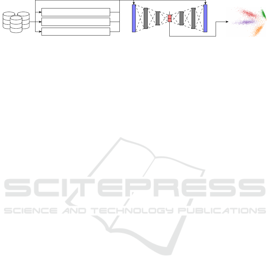
we used in our processing pipeline (Figure 2). For it,

we used standard techniques such as term frequency-

inverse document frequency transformation (tf-idf).

Additionally, we extended the pseudo-labeling ap-

proach proposed by Espadoto et al. (2021a) by com-

IVAPP 2023 - 14th International Conference on Information Visualization Theory and Applications

188

Data

Preprocessing

ﬂatten image

tf-idf transformation

pseudo-labeling

Autoencoder

Encoder Decoder

code layer

Projection

Figure 2: Our processing pipeline shows which preprocessing steps are undertaken before passing it to an autoencoder. The

code layer represents the resulting projection.

bining the cluster information with outlier informa-

tion via the Cantor pairing function.

Autoencoders. Autoencoders are a neural network

architecture belonging to the self-supervised learn-

ing algorithms class, ﬁrst presented by Hinton and

Salakhutdinov (2006). They comprise three parts:

an input layer, a set of hidden layers usually smaller

than the input layer, and an output layer of the same

size as the input layer. The inner state of the hidden

layer is called the code. Figure 2 shows the gen-

eral architecture of an autoencoder. The map that

maps the input layer to the code is called the encoder,

whereas the map that maps the hidden layer to the

output layer is called the decoder. Given a training set

D = {x

, . . . , x

} ⊆ R

, the parameters of the model

need to be adjusted in such a way that the compo-

sition g ◦ f of the encoder f : R

→ R

and the de-

coder g : R

→ R

approximates the identity map on

. This adjustment is usually made by applying the

backpropagation algorithm to the loss function

∑

i=1

− (g ◦ f )(x

))

(1)

Usually, the dimension k of the code is much smaller

than the dimension n of the input layer. Therefore

the image f (x) of a data point x ∈ R

can be seen as

a lower-dimensional representation of x. We choose

k = 2 and interpret the encoder function results as a

projection. For k = 2, the code can be visualized as a

scatter plot to explore high-dimensional datasets.

Hyperparameter Tuning. We investigate the inﬂu-

ence of hyperparameters on our researched datasets.

We restrict our considerations to the hyperparameters

which were explicitly set in the initial work of Es-

padoto et al. (2021a). We consider three kinds of hy-

perparameters: (1) hyperparameters that only inﬂu-

ence the training of the autoencoder, such as patience,

minimum delta, the number of training epochs and the

pseudo-labeling strategy, (2) backpropagation-related

hyperparameters, e.g., layer activation functions or

optimizers, and (3) architecture-related hyperparame-

ters, e.g., the number of layers. We used a grid search

for the pseudo-labeling strategy and the model archi-

tecture. For all other hyperparameters, we used a ran-

dom search.

Clustering and Outlier Mining Techniques. Clus-

tering describes ﬁnding structures of dense data points

in unlabeled data that are well separated. Speciﬁcally,

a clustering algorithm learns a discrete function that

maps similar data points to the same category (Es-

padoto et al., 2021a). Espadoto et al. (2021a) used the

k-Means algorithm (KM) and agglomerative cluster-

ing (AG) for their pseudo-labeling approach. Besides

pure clustering, we propose using labels from an out-

lier mining technique. In contrast to classical cluster-

ing, which measures the similarity between samples,

outlier mining techniques ﬁnd samples that are con-

sidered very unusual for the remaining data distribu-

tion (Liu et al., 2008).

We consider two outlier mining algorithms: Isola-

tion Forests (IF) and the Local Outlier Factor (LOF).

The LOF is an outlier mining technique focused on

the sample’s environment (Breunig et al., 2000). If a

sample is very dissimilar to its k nearest neighbors, it

is classiﬁed as an anomaly. An IF is an outlier mining

technique presented by Liu et al. (2008) that is similar

to a Random Forest. For it, an attribute is repeatedly

randomly selected and split so that, if possible, a sam-

ple is isolated. Samples that could already be isolated

with a relatively shallow depth of the tree are consid-

ered outliers. In contrast to the LOF, the global prop-

erties of the dataset are also considered (Liu et al.,

2008).

Pseudo-labels and Cantor Pairings. To provide

the autoencoder with neighborhood information, Es-

padoto et al. (2021a) provided the data points with

pseudo-labels resulting from the application of a clus-

tering algorithm. We extend this idea by sampling

different approaches to pseudo-labeling that emerge

from clustering or outlier mining algorithms. We con-

sider up to three different views on our data combined

in one pseudo-label: The top-down k-Means view,

the bottom-up agglomerative clustering view, and the

view of an outlier mining technique. All possible

combinations are listed in Table 1. By combining dif-

ferent techniques, the pseudo-labels describe a more

comprehensive view of the data. For reference, we

Evaluating Architectures and Hyperparameters of Self-supervised Network Projections

189

Table 1: List of attributes with all possible values. We only

show attributes that are subject to the random search. The

initializer values use the following abbreviations: U for uni-

form distributed and N for normal distributed.

Attribute Search Investigated parameter values

Number of epochs Random 10, 20, 30, 40, 50, 60, 70, 80, 90, 100, 200,

300, 400, 500, 600, 700, 800, 900, 1000

Patience Random 1, 2, 3, 4, 5, 6, 7, 8, 9, 10

Min. delta Random 0.01, 0.02, 0.03, 0.04, 0.05, 0.06, 0.07,

0.08, 0.09, 0.1

Clusters per class Random 1, 2, 3, 4, 5

Initializers Random Glorot U, Glorot N, random U, random N,

truncated N, He U

Layer activation

function

Random linear, tanh, sigmoid, softmax, softplus,

softsign, elu, exponential

Code layer

activation function

Random linear, tanh, sigmoid, softmax, softplus,

softsign

Optimizer Random Adam, SGD, RMSprop, Adadelta, Ada-

grad, Adamax, Nadam

L1 regularizer Random 0.0, 0.01, 0.1

L2 regularizer Random 0.0, 0.01, 0.1

Pseudo-label Grid KM, AG, KM/AG with IF/LOF, KM with

AG and IF/LOF

capture the result of a basic autoencoder without any

pseudo-labeling. For it, given the class labels x and

y from two algorithms, we create a new pseudo-label

by using the bijective Cantor pairing function (Lisi,

2007), given by:

Pair : N

→ N, (x, y) 7→

(x + y)

+ 3x + y

(2)

In the case of three labels, x, y, and z, we ap-

ply the Cantor pairing function ﬁrst on x and y

and then analogously pair the result with z, i.e.,

Pair(Pair(x, y), z).

4 EXPERIMENTS

We investigate how the hyperparameters, model ar-

chitectures, and pseudo-labels inﬂuence the result ac-

cording to our evaluation metrics. We performed two

experiments. First, we focused on how the pseudo-

labels and the training duration inﬂuenced our result.

For it, we investigated only hyperparameters that in-

ﬂuence the training but not the model deﬁnition. Our

second experiment investigates different model archi-

tectures and their related hyperparameters. We used

the SSNP implementation most recently published by

Kim et al. (2022). For more implementation details,

we refer to our auxiliary material.

Training-related Hyperparameters. In this ﬁrst

experiment, we study training-related parameters. In

detail, we will sample from four hyperparameters

with the values shown in Table 1. The number of

epochs describes how often the training data is fed

to the model. Too few epochs lead to underﬁtting

while too many epochs can result in the overﬁtting

problem without proper regularization. Patience de-

scribes a parameter that – together with the minimum

delta – inﬂuences if the training is stopped early. If

the model cannot improve over minimum delta accu-

racy over patience number of epochs the training is

stopped. The cluster per class parameter times the

number of classes determines how many cluster la-

bels are present for our cluster-based pseudo-labeling

strategy. Additionally, we perform a grid search on

the pseudo-labeling strategy. In summary, we tested

100 different parameter conﬁgurations with a random

search strategy (Bergstra and Bengio, 2012).

Backpropagation-related and Architecture-

related Hyperparameters. We test seven model

architectures with a grid search and sample

backpropagation-related hyperparameter conﬁg-

urations with values as shown in Table 1 in this

second experiment. In detail, we consider the follow-

ing hyperparameters: (1) number of layers and their

(2) number of nodes, (3) initializer, (4) layer acti-

vation function, (5) optimizer, and (6) regularizers.

A larger number of layers offers more abstraction

potential but is harder to train. The initializer sets

the initial weights and biases for each node in the

model. The layer activation function depends on the

current state of the signal from the previous layer is

fed into the next layer. For the code layer, we may

use another activation function similar to the output

layer of a neural network (Espadoto et al., 2021a).

The optimizer determines how the model weights

and biases are updated dependent on the old state

of each node and the activation function. It guides

the backpropagation of the model. Regularizers also

inﬂuence the backpropagation and systematically

force the network to not use information in order

to avoid overﬁtting. We differentiate between an l1

(linear) and l2 (quadratic) regularization. The details

of the seven model architectures can be found in the

auxiliary material. We tested ten randomly selected

parameter conﬁgurations according to the random

search strategy (Bergstra and Bengio, 2012).

Evaluation Datasets. In our experiments, we ex-

tend the datasets provided by Espadoto et al. (2021a)

by datasets provided by Atzberger et al. (2022) to val-

idate the former results and shift the focus to natural

language processing (NLP). In detail, the datasets are

given by Table 2.

IVAPP 2023 - 14th International Conference on Information Visualization Theory and Applications

190

Table 2: Details of the evaluation datasets. We use the ab-

breviation FGI for “ﬂatten grayscale image”.

Dataset

Data Points

Dimensions

Classes

Preprocessing

20-newsgroups tf-idf 16 695 23 959 20 tf-idf

ag-news tf-idf 19 175 20 860 4 tf-idf

fashion-MNIST 60 000 784 10 FGI

har 10 299 561 6 –

hatespeech tf-idf 24 783 8 176 2 tf-idf

imdb tf-idf 13 177 30 354 2 tf-idf

MNIST 60 000 784 10 FGI

reuters tf-idf 8 432 5 000 6 tf-idf

Evaluation Metrics. Here and in the following, we

always refer to the cosine distance for distance mea-

surement, as not otherwise mentioned, because – es-

pecially for very high-dimensional data – it usually

captures the similarity between data samples better

than euclidean distances (Atzberger et al., 2022). Es-

padoto et al. (2021a) used the following four metrics

for evaluating a DR:

• Trustworthiness measures the number of points

that are close to each other in the original dataset

and after projection (Espadoto et al., 2021a).

• Continuity measures the number of points that are

close to each other after projection, and which are

also close to each other in the original dataset (Es-

padoto et al., 2021a).

• The 7-Neighborhood-Hit counts how much data

points the closest seven data points in the pro-

jection have the same label as the data point

weighted by the overall presence of the label in

the dataset (Kim et al., 2022).

• The Shepard Diagram Correlation measures how

well, the dissimilarity matrix is preserved by the

DR (Joia et al., 2011).

We furthermore capture the normalized stress, which

approximates the squared error between the dissimi-

larity matrices in the high and low-dimensional space.

Those metrics focus on the neighborhood of data

samples and are therefore more concerned with lo-

cal properties of the projection. In addition, we also

measure more global properties of the data, which can

be captured by clustering metrics (Kwon et al., 2018),

speciﬁcally:

• The Calinski-Harabasz index measures the ra-

tio of the mean of inter-cluster dispersion and

the mean of intra-cluster dispersion (Cali

nski and

Harabasz, 1974). The index requires the usage of

euclidean metrics.

• The Davies-Bouldin index compares the similarity

of each cluster to its most similar cluster (Davies

and Bouldin, 1979). The index requires the usage

of euclidean metrics.

• The silhouette coefﬁcient of a data sample mea-

sures the maximal ratio between the mean dis-

tance of all data points within its cluster to the

mean distance of all data points in the next nearest

cluster (Rousseeuw, 1987).

• The s

dbw

validity index takes the cluster compact-

ness, separation, and density of clusters into ac-

count (Halkidi and Vazirgiannis, 2001).

We measured how well the data was clustered in the

original data space using their ground truth labels and

if the projection could preserve this clustering. We

normalize and invert the measurements to the [0, 1]

interval with 1 as the best possible result.

Statistical Tests. The choice of a statistical test is

dependent on the data distribution. For it, we have to

verify whether or not the quality metrics are normally

distributed. For it, we used the Quantile-Quantile-Plot

(QQ-Plot), which can be found in our auxiliary mate-

rial. The QQ-Plot reveals that the normal assumption

is invalid. We, therefore, choose statistical tests that

do not make any assumption on the underlying distri-

bution. We test two different kinds of null hypotheses:

: The pair of metric values and the increase of

a parameter occurs at random.

To verify this null hypothesis, we apply the Spear-

man correlation test (Myers and Sirois, 2004). We

can argue that the parameter signiﬁcantly inﬂuences a

metric by rejecting the null hypothesis.

: The underlying distribution of metric values

and parameter distribution is the same.

For the second null hypothesis, we use the Wilcoxon

(Gehan, 1965), the U-test (MacFarland and Yates,

2016) and the sign test (Hodges, 1955). In this case,

we aim to fail to reject the null hypothesis. In gen-

eral, this does not imply that the null hypothesis is

true but only implies insufﬁcient evidence to reject it

(Saxena et al., 2011). But in cases, where we already

rejected the ﬁrst null hypothesis and have a large sam-

ple size for each of our evaluation datasets, failing

to reject the null hypothesis consistently may provide

additional veriﬁcation that the two samples are likely

to originate from the same distribution (Makuch and

Johnson, 1986).

Evaluating Architectures and Hyperparameters of Self-supervised Network Projections

191

5 RESULTS

Our results reveal that the choice of hyperparame-

ters, especially the pseudo-labeling strategy, number

of clusters, and regularizers, can signiﬁcantly impact

the layout. Therefore, they should be chosen care-

fully. In our ﬁrst experiment, a more complex pseudo-

labeling strategy that considered outlier information

improved global metrics but decreased metrics related

to neighborhood information. In our second experi-

ment, the pseudo-labeling strategy had a weak neg-

ative correlation with the s

dbw

validity index. The

number of clusters had a modest impact on evaluation

metrics, while regularization terms were mostly neg-

atively correlated with evaluation metrics, suggesting

that no regularization is needed. The best model ar-

chitecture was found to be the one previously pro-

posed by Espadoto et al. (2021a). For the full eval-

uation material we refer to our auxiliary material.

Training-related Hyperparameters. First, consid-

ering H

, we observe that different pseudo-labeling

strategies inﬂuence the projections, as shown in Fig-

ures 1c, and 1d. The autoencoder was trained 400

epochs, using 20 clusters per class with seven epochs

and a minimum delta of 0.02 for early stopping. The

deep learning approaches differ more from non-deep

learning approaches as t-SNE, as shown in Figure 1a.

Our metrics indicate that, in this speciﬁc case, the best

pseudo-labeling strategy (besides using t-SNE) was

SSNP with KM and IF.

In the ﬁrst experiment, the number of clusters per

class and the pseudo-labeling strategy were the most

inﬂuential parameters, as shown in Table 3 (top). In-

creasing the number of clusters was correlated sig-

niﬁcantly with 8 out of 9 of our evaluation metrics

(p < 0.1%). The one metric that was correlated

without signiﬁcance was the Calinski-Harabasz in-

dex. The correlation was not positive in each case,

meaning that a higher number of clusters positively

inﬂuences the trustworthiness, continuity, Shephard

diagram correlation, silhouette coefﬁcient, Davies-

Bouldin index, and s

dbw

validity index while nega-

tively impacting the 7-neighborhood hit and the nor-

malized stress. Making the pseudo-labeling strategy

more complex was signiﬁcantly correlated to 5 out of

9 of our evaluation metrics at a signiﬁcance level of

0.1%. Again, the correlation was not positive in each

case. The pseudo-labeling strategy was positively

correlated with the Shephard diagram correlation, the

Calinski-Harabasz index, and the s

dbw

validity in-

dex. Therefore, those metrics are positively inﬂu-

enced by choosing a more complex pseudo-labeling

strategy that also considers outlier information. The

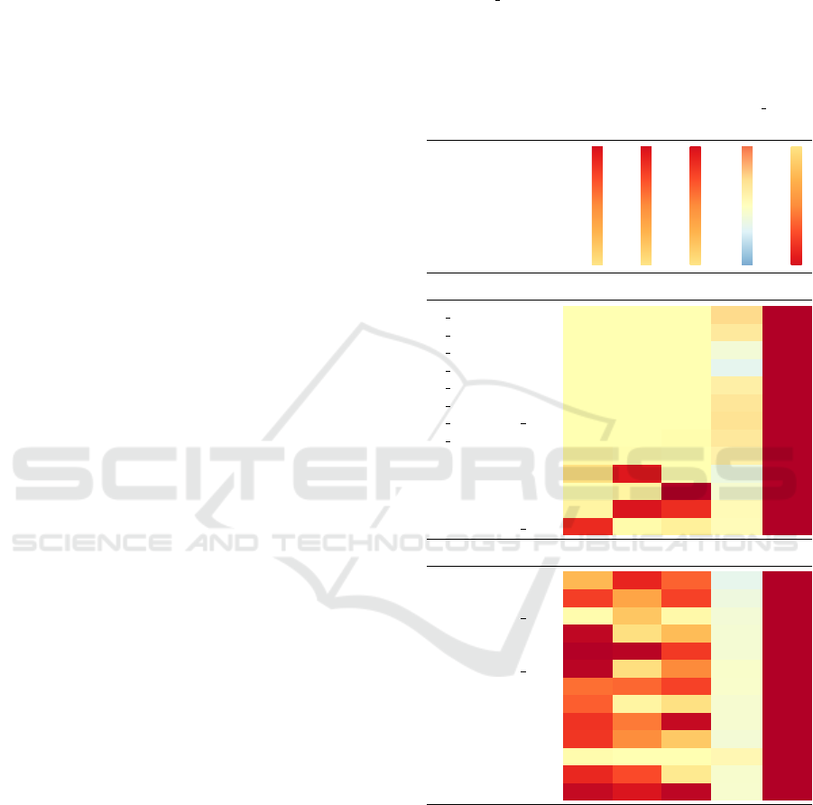
Table 3: Full list of signiﬁcantly correlated parameter-

metric pairs at signiﬁcance level 0.1% (top) and excerpt

from the signiﬁcantly correlated parameter-metric list of our

second experiment (bottom). Abbreviations: The parame-

ter value n cluster refers to the number of clusters per class,

l1 refers to l1 regularization, l2 to l2 regularization, and la-

bel to our pseudo-labeling strategy. The metric C refers to

to the continuity metric, D to the Davies-Bouldin index, H

to the Calinski-Harabasz index, N to the 7-Neighborhood

hit, S to the normalized stress, SDC to the the Shephard di-

agram correlation, SC to the silhouette coefﬁcient, s dbw to

the s

dbw

validity index and T to trustworthiness.

Parameter

Metric

Wilcoxon p

U test p

Sign test p

Spearman statistic

Spearman p

Experiment 1

n cluster C 0.00 0.00 0.00 0.36 0.00

n cluster D 0.00 0.00 0.00 0.24 0.00

n cluster N 0.00 0.00 0.00 −0.13 0.00

n cluster S 0.00 0.00 0.00 −0.27 0.00

n cluster SC 0.00 0.00 0.00 0.18 0.00

n cluster SDC 0.00 0.00 0.00 0.27 0.00

n cluster s dbw 0.00 0.00 0.00 0.30 0.00

n cluster T 0.00 0.00 0.01 0.25 0.00

label H 0.03 0.01 0.00 0.15 0.00

label N 0.13 0.85 0.00 −0.19 0.00

label S

0.00 0.04 1.00 −0.10 0.00

label SDC 0.04 0.86 0.77 0.06 0.00

label s dbw 0.78 0.02 0.06 0.04 0.00

Experiment 2

l1 C 0.31 0.80 0.61 −0.26 0.00

l1 N 0.72 0.39 0.71 −0.18 0.00

l1 s dbw 0.01 0.25 0.03 −0.13 0.00

l2 C 0.95 0.14 0.29 −0.12 0.00

l2 N 0.99 0.97 0.73 −0.12 0.00

l2 s dbw 0.97 0.14 0.51 −0.06 0.00

l2 SDC 0.58 0.60 0.71 −0.07 0.00

l2 T 0.62 0.04 0.13 −0.10 0.00

label C 0.75 0.55 0.94 −0.10 0.00

label N 0.75 0.49 0.24 −0.13 0.00

label H 0.01 0.00 0.00 0.08 0.00

label SDC 0.79 0.68 0.09 −0.08 0.00

label T 0.94 0.86 0.96 −0.09 0.00

dbw

validity index was maximized when using the

complex SSNP with KM and both AG and IF or SSNP

with KM, AG, and LOF pseudo-labeling strategy. In

contrast, the other positively correlated metrics were

mainly maximized by using the strategy that involves

KM and LOF. In contrast, the normalized stress and

the 7-neighborhood hit were negatively impacted by

choosing a more complex pseudo-labeling strategy.

The 7-neighborhood hit was optimized using a simple

pseudo-labeling strategy, and the normalized stress

IVAPP 2023 - 14th International Conference on Information Visualization Theory and Applications

192

was optimized using no pseudo-labeling strategy.

Architecture-related Hyperparameters. Consid-

ering H

, the pseudo-labeling strategy remains sig-

niﬁcant at a 0.1% signiﬁcance level for the Shephard

diagram correlation and the s

dbw

validity index. For

higher signiﬁcance levels, they also agree for patience

together with the 7-neighborhood hit or trustworthi-

ness at a signiﬁcance level of 1%. The other corre-

lation tests, especially the sign test, differ with the

remaining tests and would reject the null hypothesis

for any correlation between the number of clusters per

class and metric.

In our second experiment, we found out that the

model architecture did not signiﬁcantly correlate with

any evaluation metric for the tested parameter con-

ﬁguration for a signiﬁcance level of at least 10%.

The best results were achieved with the architecture

already proposed by Espadoto et al. (2021a). Fur-

thermore, we found out that other model-related pa-

rameters, like the amount of l1 or l2 regularization,

are (mostly negatively) signiﬁcantly correlated with

many evaluation metrics, as shown in Table 3 (bot-

tom). The amount of l1 regularization correlated sig-

niﬁcantly (p < 0.1%) with 7 out of 9 evaluation met-

rics. The l2 regularization was even for 8 out of 9

evaluation metrics (p < 0.1%). Both regularization

terms did not correlate with the Calinski-Harabasz in-

dex. The l2 regularization term additionally did not

correlate with the silhouette coefﬁcient. In contrast

to our ﬁrst experiment, our second type of hypothe-

sis test agreed with more cases of correlation found.

The l1 and l2 regularization still correlated signiﬁ-

cantly (p < 0.1%) with 5 out of 9 of our evaluation

metrics. For one up to three evaluation metrics, the

choice of the optimizer, the layer activation function,

and the initializers correlated signiﬁcantly. As before,

the pseudo-labeling strategy signiﬁcantly inﬂuenced

many evaluation parameters Table 3 (bottom). No-

tably, the choice of hyperparameters may lead to a

degenerated projection where all data points are pro-

jected around a single point, which makes the points

impossible to differentiate.

Threats to Validity. Several internal threats of va-

lidity limit the results presented above. First, we have

focused our investigations on hyperparameters that

were also present in previous work – mainly from

Espadoto et al. (2021a) – and the tested number of

hyperparameter conﬁgurations was limited by the de-

sign of our experiments. In particular, we introduced

a bias into our experiments for the chosen hyperpa-

rameter values. Second, our results are limited to the

tested data sets. Following the no-free-lunch theorem,

our results may not be applicable in another domain

for other datasets (Adam et al., 2019). Third, our

choice of statistical tests introduced further bias be-

cause three out of our four statistical tests aimed at

failing to reject the null hypothesis instead of proving

the alternative hypothesis. But following Makuch and

Johnson (1986), a reasonably large sample size would

allow us to deduce that the null hypothesis could be

true. We mitigated this bias by establishing a signif-

icant correlation according to the Spearman correla-

tion test. Furthermore, we used a reasonably large

sample size of over 200 000 samples.

External factors could also threaten our results.

First, our implementation and analysis may be sub-

ject to software bugs. However, we mitigate this risk

by inheriting publicly available source code and soft-

ware. Second, the used model relies on random num-

ber generators. We mitigated this risk by setting the

random seed everywhere applicable.

6 CONCLUSIONS

In this work, we reiterated the SSNP approach for

dimensionality reduction. For one, we extended

the original pseudo-labeling approach by consider-

ing outlier labels and pairing them with clustering la-

bels. Furthermore, we designed two experiments test-

ing different hyperparameter conﬁgurations, includ-

ing the extended pseudo-labeling approach. We mea-

sured nine evaluation metrics, i.e., ﬁve local and four

global metrics that consider local neighborhood and

global clustering properties, respectively.

Our results indicate that the architecture chosen by

Espadoto et al. (2021a) is adequate. Furthermore, the

choice of a pseudo-labeling strategy, regularization,

and the number of clusters per class inﬂuence evalu-

ation metrics signiﬁcantly. However, the correlation

is ambiguous. Most of the time, global metrics are

optimized by using a more complex pseudo-labeling

strategy while local metrics are traded-off.

We propose that future work investigates further

hyperparameter conﬁgurations, especially additional

compounded pseudo-labeling strategies. Further, we

aim to build a visualization that guides the user in

choosing a hyperparameter conﬁguration.

ACKNOWLEDGEMENTS

We thank the anonymous reviewers for their valuable

feedback. This work was partially funded by the Ger-

man Ministry for Education and Research (BMBF)

Evaluating Architectures and Hyperparameters of Self-supervised Network Projections

193

through grants 01IS20088B (“KnowhowAnalyzer”)

and 01IS22062 (“AI research group FFS-AI”).

REFERENCES

Adam, S. P., Alexandropoulos, S.-A. N., Pardalos, P. M.,

and Vrahatis, M. N. (2019). No free lunch theorem:

A review. In Approximation and Optimization: Al-

gorithms, Complexity and Applications, pages 57–82.

Springer.

Atzberger, D., Cech, T., Scheibel, W., Limberger, D.,

ollner, J., and Trapp, M. (2022). A benchmark for

the use of topic models for text visualization tasks. In

Proc. VINCI ’22, pages 17:1–4. ACM.

Becker, M., Lippel, J., Stuhlsatz, A., and Zielke, T. (2020).

Robust dimensionality reduction for data visualiza-

tion with deep neural networks. Graphical Models,

108:101060:1–15.

Bergstra, J. and Bengio, Y. (2012). Random search for

hyper-parameter optimization. JMLR, 13(10):281–

305.

Bredius, C., Tian, Z., Telea, A., Mulawade, R. N., Garth, C.,

Wiebel, A., Schlegel, U., Schiegg, S., and Keim, D. A.

(2022). Visual exploration of neural network projec-

tion stability. In Proc. MLVIS ’22, pages 1068:1–5.

EG.

Breunig, M. M., Kriegel, H.-P., Ng, R. T., and Sander, J.

(2000). LOF: Identifying density-based local outliers.

SIGMOD Record, 29(2):93–104.

Cali

nski, T. and Harabasz, J. (1974). A dendrite method

for cluster analysis. Communications in Statistics,

3(1):1–27.

Davies, D. L. and Bouldin, D. W. (1979). A cluster separa-

tion measure. TPAMI, 1(2):224–227.

Espadoto, M., Hirata, N. S., Falc

ao, A. X., and Telea, A. C.

(2020a). Improving neural network-based multidi-

mensional projections. In Proc. IVAPP ’20, pages 29–

41. INSTICC, SciTePress.

Espadoto, M., Hirata, N. S., and Telea, A. C. (2021a). Self-

supervised dimensionality reduction with neural net-

works and pseudo-labeling. In Proc. IVAPP ’21, pages

27–37. INSTICC, SciTePress.

Espadoto, M., Hirata, N. S. T., and Telea, A. C. (2020b).

Deep learning multidimensional projections. Informa-

tion Visualization, 19(3):247–269.

Espadoto, M., Martins, R. M., Kerren, A., Hirata, N. S. T.,

and Telea, A. C. (2021b). Toward a quantitative

survey of dimension reduction techniques. TVCG,

27(3):2153–2173.

Fournier, Q. and Aloise, D. (2019). Empirical comparison

between autoencoders and traditional dimensionality

reduction methods. In Proc. AIKE ’19, pages 211–

214. IEEE.

Gehan, E. A. (1965). A generalized Wilcoxon test

for comparing arbitrarily singly-censored samples.

Biometrika, 52(1–2):203–224.

Halkidi, M. and Vazirgiannis, M. (2001). Clustering validity

assessment: ﬁnding the optimal partitioning of a data

set. In Proc. ICDM ’01, pages 187–194. IEEE.

Hinton, G. E. and Salakhutdinov, R. R. (2006). Reducing

the dimensionality of data with neural networks. Sci-

ence, 313(5786):504–507.

Hodges, J. L. (1955). A bivariate sign test. The Annals of

Mathematical Statistics, 26(3):523–527.

Joia, P., Coimbra, D., Cuminato, J. A., Paulovich, F. V., and

Nonato, L. G. (2011). Local afﬁne multidimensional

projection. TVCG, 17(12):2563–2571.

Jolliffe, I. (2005). Principal component analysis. In En-

cyclopedia of Statistics in Behavioral Science. John

Wiley & Sons, Ltd.

Kim, Y., Espadoto, M., Trager, S., Roerdink, J. B., and

Telea, A. (2022). SDR-NNP: Sharpened dimension-

ality reduction with neural networks. In Proc. IVAPP

’22, pages 63–76. INSTICC, SciTePress.

Kwon, B. C., Eysenbach, B., Verma, J., Ng, K., De Filippi,

C., Stewart, W. F., and Perer, A. (2018). Clustervision:

Visual supervision of unsupervised clustering. TVCG,

24(1):142–151.

Lisi, M. (2007). Some remarks on the cantor pairing func-

tion. Le Matematiche, 62(1):55–65.

Liu, F. T., Ting, K. M., and Zhou, Z.-H. (2008). Isolation

forest. In Proc. ICDM ’08, pages 413–422. IEEE.

MacFarland, T. W. and Yates, J. M. (2016). Mann–whitney

U test. In Introduction to Nonparametric Statistics

for the Biological Sciences Using R, pages 103–132.

Springer.

Makuch, R. W. and Johnson, M. F. (1986). Some issues

in the design and interpretation of “Negative” clinical

studies. Archives of Internal Medicine, 146(5):986–

989.

McInnes, L., Healy, J., and Melville, J. (2020).

UMAP: Uniform manifold approximation and pro-

jection for dimension reduction. arXiv CoRR,

stat.ML(1802.03426). pre-print.

Myers, L. and Sirois, M. J. (2004). Spearman correlation

coefﬁcients, differences between. In Encyclopedia of

Statistical Sciences. John Wiley & Sons, Ltd.

Rousseeuw, P. J. (1987). Silhouettes: A graphical aid to

the interpretation and validation of cluster analysis.

Journal of Computational and Applied Mathematics,

20:53–65.

Saxena, D., Yadav, P., and Kantharia, N. (2011). Nonsignif-

icant P values cannot prove null hypothesis: Absence

of evidence is not evidence of absence. Journal of

Pharmacy and Bioallied Sciences, 3(3):465–466.

van der Maaten, L. and Hinton, G. (2008). Visualizing data

using t-SNE. JMLR, 9(11):2579–2605.

Yang, L. and Shami, A. (2020). On hyperparameter opti-

mization of machine learning algorithms: Theory and

practice. Neurocomputing, 415:295–316.

APPENDIX

The auxiliary material is available under 10.5281/zen-

odo.7501914 and contains implementation details,

the QQ-Plots, and all evaluation results.

IVAPP 2023 - 14th International Conference on Information Visualization Theory and Applications

194