Image Generation from a Hyper Scene Graph
with Trinomial Hyperedges
Ryosuke Miyake, Tetsu Matsukawa
a
and Einoshin Suzuki
b
Graduate School and Faculty of Information Science and Electrical Engineering, Kyushu University, Fukuoka, Japan
Keywords:
Image Generation, Scene Graph, Hyper Graph, Generative Adversarial Network.
Abstract:
Generating realistic images is one of the important problems in the field of computer vision. In image genera-
tion tasks, generating images consistent with an input given by the user is called conditional image generation.
Due to the recent advances in generating high-quality images with Generative Adversarial Networks, many
conditional image generation models have been proposed, such as text-to-image, scene-graph-to-image, and
layout-to-image models. Among them, scene-graph-to-image models have the advantage of generating an
image for a complex situation according to the structure of a scene graph. However, existing scene-graph-to-
image models have difficulty in capturing positional relations among three or more objects since a scene graph
can only represent relations between two objects. In this paper, we propose a novel image generation model
which addresses this shortcoming by generating images from a hyper scene graph with trinomial edges. We
also use a layout-to-image model supplementally to generate higher resolution images. Experimental valida-
tions on COCO-Stuff and Visual Genome datasets show that the proposed model generates more natural and
faithful images to user’s inputs than a cutting-edge scene-graph-to-image model.
1 INTRODUCTION
Generating realistic images is one of the important
problems in the field of computer vision. Image
generation can be applied in various fields (Agnese
et al., 2020; Wu et al., 2017) such as medicine (Nie
et al., 2017; Ghorbani et al., 2020) and art (Elgam-
mal et al., 2017). In the field of art, it could be
useful for artists and graphic designers. In the fu-
ture, when higher-quality images can be generated,
image or video search engines can be replaced by al-
gorithms which generate customized content based on
user preferences (Johnson et al., 2018).
In image generation tasks, generating images con-
sistent with the input given by the user is called condi-
tional image generation. In recent years, advances in
research on Generative Adversarial Networks (GAN),
(Goodfellow et al., 2014) have improved the qual-
ity of generated images, and many conditional image
generation models have been proposed. Among them,
text-to-image models (Reed et al., 2016; Zhang et al.,
2017; Zhang et al., 2018; Odena et al., 2017) gener-
ate images conditioned on a text such as “the sheep
is on the grass”. These models have the advantage
a
https://orcid.org/0000-0002-8841-6304
b
https://orcid.org/0000-0001-7743-6177
of their simple input and their ease of application in
many fields. Meanwhile, they have the disadvantage
of their difficulty in generating images which repre-
sent complex situations with many objects and their
relations. This drawback is attributed to the difficulty
in generating a single feature vector which contains
all of the information in a long sentence.
A scene graph represents situations in a similar
way to a text (Johnson et al., 2015). It consists of
nodes representing objects such as “dog” and bino-
mial edges representing a relation between two ob-
jects such as “on”. In the scene-graph-to-image mod-
els, each object or edge label in a scene graph is trans-
formed into a feature vector. In other words, text-to-
image models convert a sentence into a feature vector,
while scene-graph-to-image models generate feature
vectors from each word in a scene graph. Thus, en-
coding a scene graph into a feature vector is easier,
and this fact enables these models to generate proper
images for complex situations.
Though scene-graph-to-image models have such
an advantage, they have a shortcoming: the positional
relations among three or more objects tend to be inac-
curate (Figure1 (a)). An edge in a scene graph can
represent only relations between two objects, so it
has difficulty in capturing a positional relation among
three or more objects. This inaccurate object position-
Miyake, R., Matsukawa, T. and Suzuki, E.
Image Generation from a Hyper Scene Graph with Trinomial Hyperedges.
DOI: 10.5220/0011699300003417
In Proceedings of the 18th International Joint Conference on Computer Vision, Imaging and Computer Graphics Theory and Applications (VISIGRAPP 2023) - Volume 5: VISAPP, pages
185-195
ISBN: 978-989-758-634-7; ISSN: 2184-4321
Copyright
c
 2023 by SCITEPRESS – Science and Technology Publications, Lda. Under CC license (CC BY-NC-ND 4.0)
185

ing also causes overlapping of positions of the gen-
erated objects, which causes another shortcoming of
generating unclear objects (Figure 1 (b)).
We address the former shortcoming by generat-
ing images from the hyper scene graph with trinomial
hyperedges each of which represents the positional
relation among three objects. If the shortcoming of
the positional relationship is improved with hyper-
edges, the object overlapping is reduced, resulting in
sharper objects and images. Moreover, we use layout-
to-image model Layout2img (He et al., 2021) supple-
mentally to generate high resolution images.
Scene Graph
(a)
Layout
Image
(b)
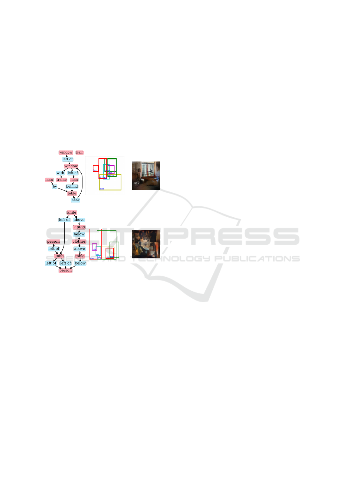
Figure 1: Example of scene-graph-to-model sg2im (John-
son et al., 2018) failing to generate images which are not
consistent with the input. The layout in the second column
is the intermediate product of sg2im. The scene graph in
(a) has a path “window” (green bounding box) → “left of”
→ “man” (purple). However, in the generated layout, “win-
dow” (green) surround “man” (purple) and is not positioned
in the left of “man” (purple). In the generated image in (b),
the entire image is unclear, and thus it is difficult to insist
that the objects in the scene graph are generated.
2 RELATED WORKS
Image generation models fall into three categories: (i)
GAN (Goodfellow et al., 2014; Radford et al., 2015),
(ii) VAE (Kingma and Welling, 2013), and (iii) au-
toregressive models (Van Den Oord et al., 2016). (i)
A GAN consists of a generator G and a discrimina-
tor D. The generator generates data x
′
from noise z
sampled from noise distribution p
z
. The discriminator
outputs the probability that the given data is not x
′
but
x sampled from the training data. These two models
are trained to compete with each other. (ii) VAE con-
sists of an encoder and a decoder. The encoder takes
an image as input and outputs a latent variable. The
decoder aims to recover the original image from the
latent variable. The two networks are trained simul-
taneously. (iii) The autoregressive model generates
an image by sequentially generating the value of each
pixel conditioned on all previously generated pixels.
In these three models, GAN is widely used in con-
ditional image generation models due to the realistic
look of the generated images and its ease of applica-
tion to various models. In this paper, we also employ
GAN as the generative model.
Major inputs for conditional image generation
models using GAN are (1) text (Reed et al., 2016;
Zhang et al., 2017; Zhang et al., 2018; Odena et al.,
2017), (2) layouts (Sun and Wu, 2019; He et al., 2021;
Hinz et al., 2019; Hinz et al., 2022), and (3) scene
graphs (Johnson et al., 2018; Li et al., 2019; Vo and
Sugimoto, 2020; Mittal et al., 2019). In the following,
we categorize each generative model by these three
kinds of inputs and explain them.
(1) The text-to-image models have been studied
extensively due to their advantages of their simple in-
put and their ease of application in many fields. Reed
et al. extended cGAN (Mirza and Osindero, 2014)
to generate images which are aligned with the input
semantically by using GAN-INT-CLS (Reed et al.,
2016). Odena et al. proposed AC-GAN (Odena
et al., 2017), in which the discriminator solves a task
of identifying the class of a given image in addition
to the general discriminative problem, and tried to
generate images where each object can be identified.
These models can generate an image consistent with
the input for a simple situation which involves few ob-
jects and few relations. However, they have difficulty
in generating images representing complex situations
with many objects and relations between them.
(2) Layout-to-image models and (3) scene-graph-
to-image models were proposed to overcome the
shortcoming of text-to-image models (Johnson et al.,
2018; Hinz et al., 2019). (2) He et al. proposed a
layout-to-image model Layout2img (He et al., 2021).
This model generates consistent feature vectors for
each object and generates natural images. The layout-
to-image models can control the position of the gen-
erated object directly by the input. On the other hand,
they have difficulty in being applied to image gener-
ation from a text due to the dissimilarity of the struc-
tures between a text and a layout.
(3) Johnson et al. proposed a scene-graph-to-
image model sg2im (Johnson et al., 2018). This
VISAPP 2023 - 18th International Conference on Computer Vision Theory and Applications
186

model processes a scene graph using a graph convo-
lutional network. Compared with the text-to-image
model StackGAN (Zhang et al., 2017), sg2im gener-
ates images which are semantically more consistent
with the input. Scene-graph-to-image models pos-
sess two main advantages, i.e., the ease of convert-
ing the input to a feature vector and the ease of ap-
plying them to text-to-image models. The former is
due to their ease of making feature vectors. A text-to-
image model converts an entire sentence into a feature
vector, while a scene-graph-to-image model converts
each word into a feature vector. The latter is attributed
to the similarity of the structures between a text and a
scene graph. Actually, there is research on the trans-
formation from a text to a scene graph (Schuster et al.,
2015). On the other hand, as explained in Section 1,
the scene-graph-to-image model has difficulty in cap-
turing the positional relations among three or more
objects correctly.
In this paper, we focus on scene-graph-to-image
models due to their advantages and aim to overcome
its shortcoming. In addition, we use the layout-to-
image model as a supplement to generate higher res-
olution images.
3 TARGET PROBLEM
To make the distinction between Johnson et al.’s work
and ours clear, first, we explain their target problem
(Johnson et al., 2018): image generation from a scene
graph. Then, we describe our target problem: image
generation from a hyper scene graph, and the evalua-
tion metrics used in this paper.
3.1 Image Generation from a Scene
Graph
Johnson et al. set the target problem to creating gen-
erator G(S, z) which generates image
ˆ
I from scene
graph S = (V, E) and Gaussian noise z. Each object
v
i
∈ V has a category such as “dog” and “sky”. V de-
notes the set of nodes in the scene graph, where V =
{v
1
, . . . , v
n
}, and n represents the number of nodes. A
node represents an object. Category c
i
∈ C of object
v
i
is denoted by c
i
= f (v
i
), where C is the set of all
categories of objects and f (·) is a mapping from ob-
ject v ∈ V to category c ∈ C of objects. E denotes
the set of binomial edges in a scene graph, satisfy-
ing E ⊆ V × R
2
×V , where R
2
is the entire set of la-
bels for binomial relations (“on”, “left of”, etc.). Note
that for (v
i
, r
j
, v
k
) ∈ E, i ̸= k. A binomial edge is di-
rected: (v
i
, r
j
, v
k
) and (v
k
, r
j
, v
i
) are distinct. Figure 2
(a) shows an example of a scene graph.
3.2 Image Generation from a Hyper
Scene Graph
We define the hyper scene graph as a scene graph
with an additional hyperedge that represents a rela-
tion among three or more objects. In this paper,
we focus on relations among three objects for sim-
plicity. As described in Section 1, sg2im (Johnson
et al., 2018) has a shortcoming: the positional re-
lations in the generated image among three or more
objects tend to be inaccurate. To address this short-
coming, we set our target problem to creating gen-
erator G(H,z) which generates image
ˆ
I from hy-
per scene graph H = (V, E, Q) and Gaussian noise
z. Q denotes the set of trinomial hyperdeges in
H, which satisfies Q ⊆ V × R
3
× V × V . R
3
de-
notes the entire set of labels (such as “between”)
for the trinomial relation. Trinomial hyperedge
(v
i
, r
j
, v
k
, v
l
) ∈ Q satisfies i ̸= k, i ̸= l, k ̸= l and
is directed: (v
i
, r
j
, v
k
, v
l
), (v
i
, r
j
, v
l
, v
k
), (v
l
, r
j
, v
i
, v
k
),
(v
l
, r
j
, v
k
, v
i
), (v
k
, r
j
, v
i
, v
l
), and (v
k
, r
j
, v
l
, v
i
) are dis-
tinct. The definitions of V and E are the same as in
Section 3.1. Figure 2 (b) shows an example of a hyper
scene graph.
(a)
(b)
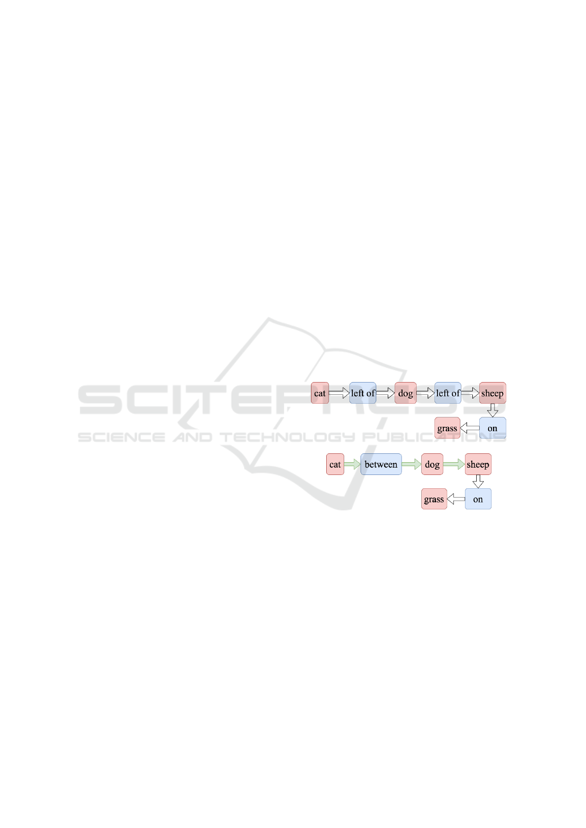
Figure 2: Example of a scene graph (a) and a hyper
scene graph (b). The red box and blue box represent
an object and an edge label, respectively. The white
arrow and green arrow represent a binomial edge and
a trinomial hyperedge, respectively. Set V of objects
and category f (V ) of objects are the same in both (a)
and (b), and they are given by V = {v
1
, v
2
, v
3
, v
4
},
f (V) = {“cat”, “dog”, “sheep”, “grass”}. Set E
a
and E
b
of
binomial edges are given by E
a
= {(v
1
, r
1
(“left of”), v
2
),
(v
2
, r
2
(“left of”), v
3
), (v
3
, r
3
(“on”), v
4
)} and
E
b
= {(v
3
, r
3
(“on”), v
4
)}, respectively. Set Q
b
of trinomial
hypereges is given by Q
b
= {(v
1
, r
4
(“between”), v
2
, v
3
)}.
The path “cat” → “left of” → “dog” corresponds to the
binomial edge (v
1
(“cat”)), “left of”, v
2
(“dog”)) and means
that a cat exists to the left of a dog. Also, the path “cat” →
“between ” → “dog” → “sheep” corresponds to the trino-
mial edge (v
1
(“cat”)), “between”, v
2
(“dog”), v
2
(“sheep”))
and means from left to right, a cat, a dog, and a sheep align
in a row.
Image Generation from a Hyper Scene Graph with Trinomial Hyperedges
187

3.3 Evaluation Metrics
There are various evaluation measures for conditional
image generation models, such as the fidelity and the
diversity of the generated images to the input, the
clarity of the boundaries, and the robustness to small
changes in the input (Frolov et al., 2021). In this pa-
per, we aim to achieve the following three goals.
A). Improving the positional relation among three ob-
jects connected to a hyperedge.
B). Making the overlapping of the objects small.
C). Making the generated image natural.
As the evaluation metrics for (A)∼(C), we use
Positional relation of Three Objects (PTO), Area of
Overlapping (AoO), and Inception Score (Salimans
et al., 2016), respectively. PTO and AoO are new
measures proposed in this paper. As an evaluation
measure for (C), we could also use the Fr
´
echet In-
ception Distance (FID) (Heusel et al., 2017), which
is the distance between the distribution of the embed-
ded representations of the real images and the gener-
ated images. However, we use Inception Score in line
with (Johnson et al., 2018) in this paper.
PTO is the percentage of correctly generating
three bounding boxes b
i
, b
j
, b
k
for v
i
, v
j
, v
k
satisfying
(v
i
, “between”, v
j
, v
k
) ∈Q. We judge that bounding
boxes b
i
, b
j
, b
k
are correctly generated if they satisfy
the following five conditions for the addition of a tri-
nomial hyperedge “between”.
• v
i
, v
j
, v
k
are lined up from left to right in this order,
where each of objects does not overlapping, i.e.,
x
i0
< x
i1
< x
j0
< x
j1
< x
k0
< x
k1
.
• v
i
, v
j
, v
k
are not large objects such as the back-
ground, i.e., x
i1
− x
i0
< 0.7w and x
k1
− x
k0
< 0.7w
and x
k1
−x
k0
< 0.7w, where w is the image width.
• v
i
, v
j
, v
k
are of nearly equal size, i.e.,
1
2
<
x
i1
−x
i0
x
j1
−x
j0
< 2 and
1
2
<
y
i1
−y
i0
y
j1
−y
j0
< 2 and
1
2
<
x
j1
−x
j0
x
k1
−x
k0
< 2 and
1
2
<
y
j1
−y
j0
y
k1
−y
k0
< 2.
• v
i
, v
j
, v
k
are not largely apart horizontally,
i.e., max(x
i1
− x
i0
, x
j1
− x
j0
)0.5 > x
j0
− x
i1
and
max(x
j1
− x
j0
, x
k1
− x
k0
)0.5 > x
k0
− x
j1
.
• v
i
, v
j
, v
k
are not largely apart vertically, i.e.,
max(y
i1
− y
i0
, y
j1
− y
j0
)0.7 > y
j0
− y
i1
and
max(y
j1
− y
j0
, y
k1
− y
k0
)0.7 > y
k0
− y
j1
.
Here, b
i
= (x
i0
, x
i1
, y
i0
, y
i1
), (x
i0
< x
i1
, y
i0
< y
i1
),
which means that the bounding box is a rectangle with
vertices (x
i0
, y
i0
), (x
i0
, y
i1
), (x
i1
, y
i0
), (x
i1
, y
i1
). PTO is
defined by
PTO =
the number of correctly generated sets
the number of the evaluated sets
. (1)
For sg2im (Johnson et al., 2018), which employs no
hyperedges, we evaluate whether objects (v
i
, v
j
, v
k
)
satisfy (v
i
, “left of”, v
j
) and (v
i
, “left of”, v
j
) ∈ E.
AoO examines whether the introduction of the tri-
nomial hyperedge reduces the overlapping of objects.
AoU measures the overlapping of three objects con-
nected to a trinomial hyperedge. AoU is defined as
follows.
AoO(b
i
, b
j
, b
k
) =
IoU(b
i
, b
j
) + IoU(b
i
, b
k
) + IoU(b
j
, b
k
) (2)
where IoU (Intersection over Union) (Rezatofighi
et al., 2019) is a measure for evaluating the overlap-
ping of two bounding boxes. IoU has been used to
evaluate the overlapping of generated boxes and the
ground truth boxes in the dataset. However, our ob-
jective is to improve the relative position between the
generated bounding boxes as we explained in Section
1. Thus, we use IoU for the evaluation of the over-
lapping of three objects here. Let the two bounding
boxes be X, Y and S(·) be the area of the input region.
Then, IoU is defined as follows.
IoU(X,Y ) =
S(X ∩Y)
S(X ∪Y)
(3)
The smaller AoO is, the smaller the overlapping be-
tween the objects is, which indicates that the objects
are generated with appropriate positioning. In sg2im,
we evaluate whether the bounding boxes of v
i
, v
j
, v
k
satisfy (v
i
, “left of”, v
j
), (v
i
, “left of”, v
j
) ∈ E.
We use Inception Score (IS) (Salimans et al.,
2016) as a measure for evaluating the naturalness of
the generated image. IS is calculated using Inception
Network trained on ImageNet (Russakovsky et al.,
2015; Szegedy et al., 2015) with the following equa-
tions.
IS = exp[E
ˆ
I
[D
KL
(p(y|
ˆ
I)∥p(y)]], (4)
p(y) =
1
N
N
∑
i=1
p(y|
ˆ
I
i
), (5)
where p(y|
ˆ
I) is the probability of label y of input im-
age
ˆ
I predicted by Inception Network and p(y) is its
marginal probability. The score becomes larger when
the labels of the generated images are easily identi-
fied and the identified labels are diverse. Therefore,
we can use Inception Score as the evaluation measure
for the naturalness of the generated image.
4 ORIGINAL MODEL
We design our model based on an image generation
model from a scene graph sg2im (Johnson et al.,
2018). In this Section, we explain sg2im (Johnson
et al., 2018) and its shortcoming.
VISAPP 2023 - 18th International Conference on Computer Vision Theory and Applications
188

4.1 sg2im (Johnson et al., 2018)
First, we show an overview of generator G of sg2im
(Johnson et al., 2018) in Figure 3 (a). In the gener-
ator of sg2im, a hyper scene graph is a scene graph,
the hyper graph convolutional network is the graph
convolutional network, a layout is a feature map, and
Layout2img is Cascaded Refinement Network (Chen
and Koltun, 2017). The image generation in the gen-
eration phase is performed as follows.
1. Each v ∈ V of the objects and binomial relation
labels r ((·, r, ·) ∈ E) in scene graph S is trans-
formed into object vector ν and relation vector ρ
by the object embedding network and the relation
embedding network, respectively.
2. We apply graph convolution on object vector ν
and relation vector ρ based on scene graph S and
obtain convoluted object vectors.
3. The box regression network is applied to the con-
voluted object vectors to predict bounding box
ˆ
B
which represents the region to generate each ob-
ject.
4. We generate feature map M, which is an interme-
diate representation between a scene graph and an
image region, by mapping the convoluted object
vectors based on their bounding boxes
ˆ
B.
5. Feature map M with Gaussian noise z is fed
into the Cascaded Refinement Network (Chen and
Koltun, 2017) to generate image
ˆ
I.
The graph convolution in step 2 is performed to
convert the feature vector of each object so that it
considers the entire scene graph. Figure 4 shows
the process flow of the first layer of the graph con-
volution network when the scene graph in Figure 2
(a) is the input. net1 is a multi-layer perceptron ap-
plied to binomial relations, which takes as input vec-
tors (ν
i
, ρ
j
, ν
k
) corresponding to e = (v
i
, r
j
, v
k
) ∈ E,
(r
j
∈ R
2
) and outputs vectors (ν
i j
, ρ
′
j
, ν
k j
). Then,
pooling and dimensionality reduction by net2 are per-
formed for each object vector, and the first layer of
the graph convolution is completed. The graph con-
volution network has five layers, and the output of the
previous layer is used as the input to the next layer.
By repeating this process, information on each ob-
ject vector and relation vector is propagated along the
edges.
Next, we describe the discriminators. In sg2im
(Johnson et al., 2018), there are two discriminators:
D
img
and D
ob j
. D
img
takes a generated image or a
training image as input and outputs the probability
that the input is a generated image. D
ob j
takes as input
a generated object in the generated image or an object
in the dataset image and outputs the probability that
the input is a generated object and the probability that
its category is c ∈ C . By identifying the category of
each object with D
ob j
, we can learn the semantic con-
sistency between the word and the image.
4.2 Shortcomings of sg2im (Johnson
et al., 2018)
As described in Section 1, sg2im (Johnson et al.,
2018) has a shortcoming: the positional relations
among three or more objects tend to be inaccurate.
The edges in a scene graph can represent only rela-
tions between two objects. Therefore, a multilayer
perceptron (MLP) in the graph convolution network is
applied to the features of three objects in two separate
steps. For example, for a path “cat” → “left of” →
“dog” →“left of” → “sheep” in the scene graph, the
convolution is performed on the two edges “cat” →
“left of” → “dog” and “dog” → “left of” → “sheep”.
This fact leads to the difficulty of sg2im in capturing
the positional relations among three or more objects.
Moreover, sg2im (Johnson et al., 2018) has diffi-
culty in generating the objects clearly due to the low
resolution (64×64) of the generated images when the
input scene graph involves many objects. We con-
firmed that simply increasing the resolution of the
generated images does not work well due to the mode
collapse (Gui et al., 2021), which is a phenomenon
that the generated images are all similar to each other
due to the training failure.
5 PROPOSED MODEL
To address the shortcoming of the existing image gen-
eration model from a scene graph, we propose an
image generation model from a hyper scene graph
hsg2im. In this Section, we explain the proposed
model hsg2im, and training of hsg2im.
5.1 hsg2im
As explained in Section 1, sg2im (Johnson et al.,
2018) has a shortcoming: the positional relations
among three objects tend to be inaccurate due to the
convolution method.
We address this shortcoming by modifying two
parts from sg2im (Johnson et al., 2018): generating
images from a hyper scene graph with a trinomial
hyperedge and extending the graph convolution net-
work to the hypergraph convolution network. Also, to
generate a higher resolution image, we use a layout-
to-image model Layout2img (He et al., 2021). Lay-
out2img generates images whose resolution is 128
Image Generation from a Hyper Scene Graph with Trinomial Hyperedges
189

×128. In this Section, we explain image generation
using the hypergraph convolution network and Lay-
out2img (He et al., 2021). An overview of the gener-
ator G of hsg2im is shown in Figure 3 (b). The dis-
criminator is unchanged from that of sg2im.
First, we create the hypergraph convolution net-
work by adding a multi-layer perceptron net3, which
is applied to trinomial hyperedges, to the graph con-
volution network of sg2im. The net3 takes vectors
(ν
i
, ρ
j
, ν
k
, ν
l
) as input and outputs vectors (ν
i j
, ρ
′
j
,
ν
k j
, ν
l j
) corresponding to a trinomial hyperedge q =
(v
i
, r
j
, v
k
, v
l
) ∈ Q. The addition of net3 enables the
convolution of the hyper scene graph with trinomial
hyperedges. As a result, three objects are processed
with an application of net3 and two applications of
net1, and their positional relation is expected to be im-
proved. Furthermore, the improved positional relation
reduces the overlapping of objects and is expected to
produce more consistent layouts with the input, which
leads to generating better images. Figure 4 shows the
application of the hypergraph convolution network to
the hyper scene graph in Figure 2 (b).
Next, we describe image generation using Lay-
out2img (He et al., 2021). To address the image res-
olution shortcoming of sg2im, we use the pre-trained
model Layout2img, which generates a 128×128 im-
age from layout L = {(c
i
, b
i
)}
N
i=1
, as an auxiliary
model. {(c
i
)}
N
i=1
is obtained from the input (hyper)
scene graph. Bounding box
ˆ
B = {(b
i
)}
N
i=1
is gen-
erated in the framework of sg2im (Johnson et al.,
2018) with the hypergraph convolutional neural net-
work. Layout2img uses the structure of ResNet (He
et al., 2016) in its generator, so that even models
which generate a high resolution image (128 × 128)
can be trained stably.
5.2 Training of hsg2im
The training of generator G and discriminator D is
performed alternately. During the training phase, fea-
ture map M is created from bounding box B in the
dataset. Loss L
G
of generator G is L
G
=
∑
5
i=1
w
i
L
i
,
where w
i
is the weight of loss L
i
defined as follows.
• Loss with respect to image pixels: L
1
= L
pix
• Loss with respect to the bounding box: L
2
= L
box
• Adversarial loss from discriminator D
img
: L
3
=
L
img
GAN
• Adversarial loss from discriminator D
obj
: L
4
=
L
obj
GAN
• Auxiliarly classifier loss from D
obj
: L
5
= L
obj
AC
The losses (L
pix
, L
box
, L
img
GAN
, L
obj
GAN
, L
obj
AC
) and their
weights set are the same as in (Johnson et al., 2018).
6 EXPERIMENTS
6.1 Dataset
We use as datasets the 2017 COCO Stuff (Caesar
et al., 2018) and Visual Genome (Krishna et al., 2017)
by adding trinomial hyperedges. The 2017 COCO-
Stuff dataset (COCO) (Caesar et al., 2018) consists
of images, objects, their bounding boxes, and seg-
mentation masks. There are 40,000 training images
and 5,000 validation images. Since the COCO dataset
does not contain data on relations between objects, we
construct a hyper scene graph by adding seven rela-
tions “left of”, “right of”, “above”, “below”, “inside”,
“surrounding”, and “between” based on the bounding
boxes. The “between” relation is added as a trinomial
hyperedge in hsg2im. Since there is no test set in the
COCO dataset, we divide the validation set into a new
validation set and a test set. As a result, the COCO
dataset contains 24,972 training images, 1,667 vali-
dation images, and 3,333 test images.
The Visual Genome (Krishna et al., 2017) version
1.4 (VG) dataset, consisting of 108,077 images anno-
tated with scene graphs, consists of images, objects,
their bounding boxes, and the binomial relations be-
tween the objects. In the entire dataset, only objects
which appear more than 2,000 times and relations
which appear more than 500 times are used following
(Johnson et al., 2018) in our experiments. Samples
with less than 2 objects and more than 31 objects are
ignored. As a result, we use 62,602 training images,
5,069 evaluation images, and 5,110 test images. For
Visual Genome, we add the “between” relation (4,136
hyperedges) as in COCO.
In addition, to compare sg2im with our hsg2im,
we also add the binomial edges “left of” (8,272
edges) corresponding to hyperedges “between” in
both datasets: (v
i
, “left of”, v
j
) and (v
j
, “left of”, v
k
),
together which correspond to (v
i
, “between”, v
j
, v
k
).
Next, we explain how to add hyperedges “be-
tween” and “left of”. For hsg2im, both a trino-
mial hyperedge (v
i
, “between”, v
j
, v
k
) and two bino-
mial edges (v
i
, “left of”, v
j
) and (v
i
, “left of”, v
j
) are
added for three objects (v
i
, b
i
), (v
j
, b
j
), (v
k
, b
k
) which
satisfy all of the five conditions in Section 3.3. For
sg2im, only the latter two are added. In Visual
Genome, we add 3,477 hyperedges, 334 hyperedges,
and 325 hyperedges for the training dataset, the val-
idation dataset, and the test dataset, respectively. In
COCO, we add 9,437 hyperedges, 144 hyperedges,
and 227 hyperedges for the training dataset, the vali-
dation dataset, and the test dataset, respectively.
VISAPP 2023 - 18th International Conference on Computer Vision Theory and Applications
190

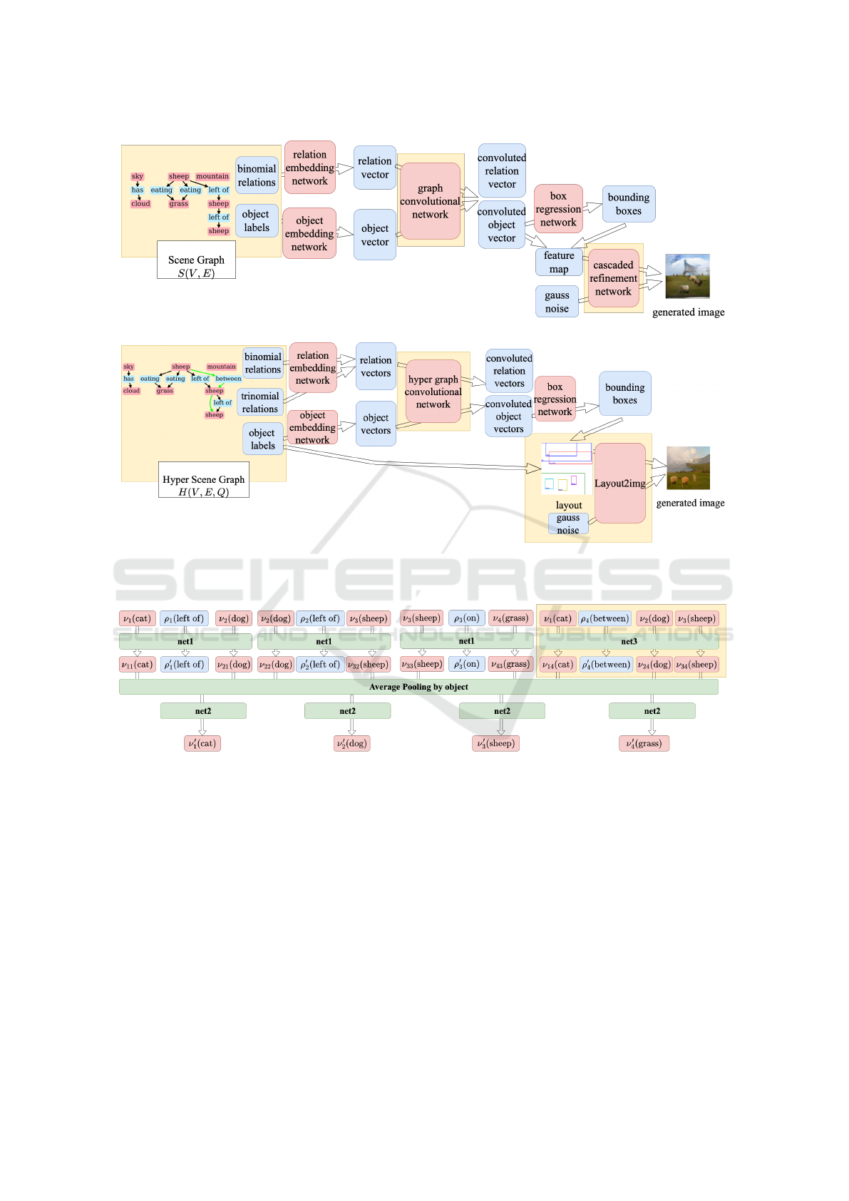
(a)
(b)
Figure 3: Example of generating an image not using Layout2img (He et al., 2021) with generator G of sg2im (Johnson et al.,
2018) (a) and using Layout2img with generator G of hsg2im (b). The elements that we modified are highlighted in yellow.
Figure 4: Flowchart of one of the five layers of the hyper graph convolutional network of hsg2im. The part without the yellow
region shows that of the graph convolutional network of sg2im (Johnson et al., 2018). net1, net2, and net3 represent MLPs
for binomial edges, dimension reduction, and trinomial hyperedges, respectively. The detailed structures of net1, net2, and
net3 are given in APPENDIX.
6.2 Experimental Conditions
We train sg2im and hsg2im on the COCO and Visual
Genome datasets, respectively, based on the method
described in Section 5.2. Here, the learning algorithm
(Adam (Kingma and Ba, 2015) ), the learning rate
(= 10
−4
), the batch size (= 32), and the iteration up-
per bound (= 10
6
) are the same as in the sg2im paper
(Johnson et al., 2018).
6.3 Results and Discussion
First, we quantitatively evaluate hsg2im. The evalua-
tion in terms of PTO is shown in Table 1. We see that
hsg2im shows 12% and 20% higher scores than s2im
on the COCO and VG datasets, respectively. These
results are because the trinomial hyperedge enables
us to capture the positional relations among three ob-
jects.
We show the evaluation in terms of AoO in Table
2. hsg2im shows a higher score on the VG dataset.
Image Generation from a Hyper Scene Graph with Trinomial Hyperedges
191

Table 1: Comparison of PTO scores between sg2im and
hsg2im.
COCO VG
sg2im 0.52 0.19
hsg2im 0.64 0.39
In the COCO dataset, the scores of sg2im and hsg2im
are the same. We speculate that the identical scores
on the COCO dataset are due to the few diversity
of binomial edges on this dataset; sg2im generated
fewer overlapping bounding boxes only with bino-
mial relations. Therefore, the room for improvement
is small. For VG, we can confirm that the addition of a
trinomial hyperedge improves the positional relation
of three objects and reduces the overlapping between
them.
Table 2: Comparison of AoO scores between sg2im and
hsg2im.
COCO VG
sg2im 0.02 0.11
hsg2im 0.02 0.06
We show the evaluation in terms of Inception
Score in Table 3. In the image generated without Lay-
out2img, hsg2im shows a 0.33 lower score for COCO
and a 0.40 higher score than sg2im for Visual Genome
datasets. For images generated using Layout2img,
hsg2im shows 0.26 and 0.10 higher scores than sg2im
for COCO and Visual Genome datasets, respectively.
In the case of not using Layout2img for COCO, the
reason of the degraded IS would be attributed to the
lowness of the resolution. Overall, the scores show
that the images generated with Layout2img are more
natural than those generated by sg2im and more nat-
ural images are generated from layouts produced by
hsg2im than by sg2im.
Table 3: Comparison of Inception Score between sg2im and
hsg2im, and with and without Layout2img.
COCO VG
sg2im 4.17 5.45
hsg2im wo Layout2img 3.84 5.85
sg2im + Layout2img 11.63 9.83
hsg2im + Layout2img 11.89 9.93
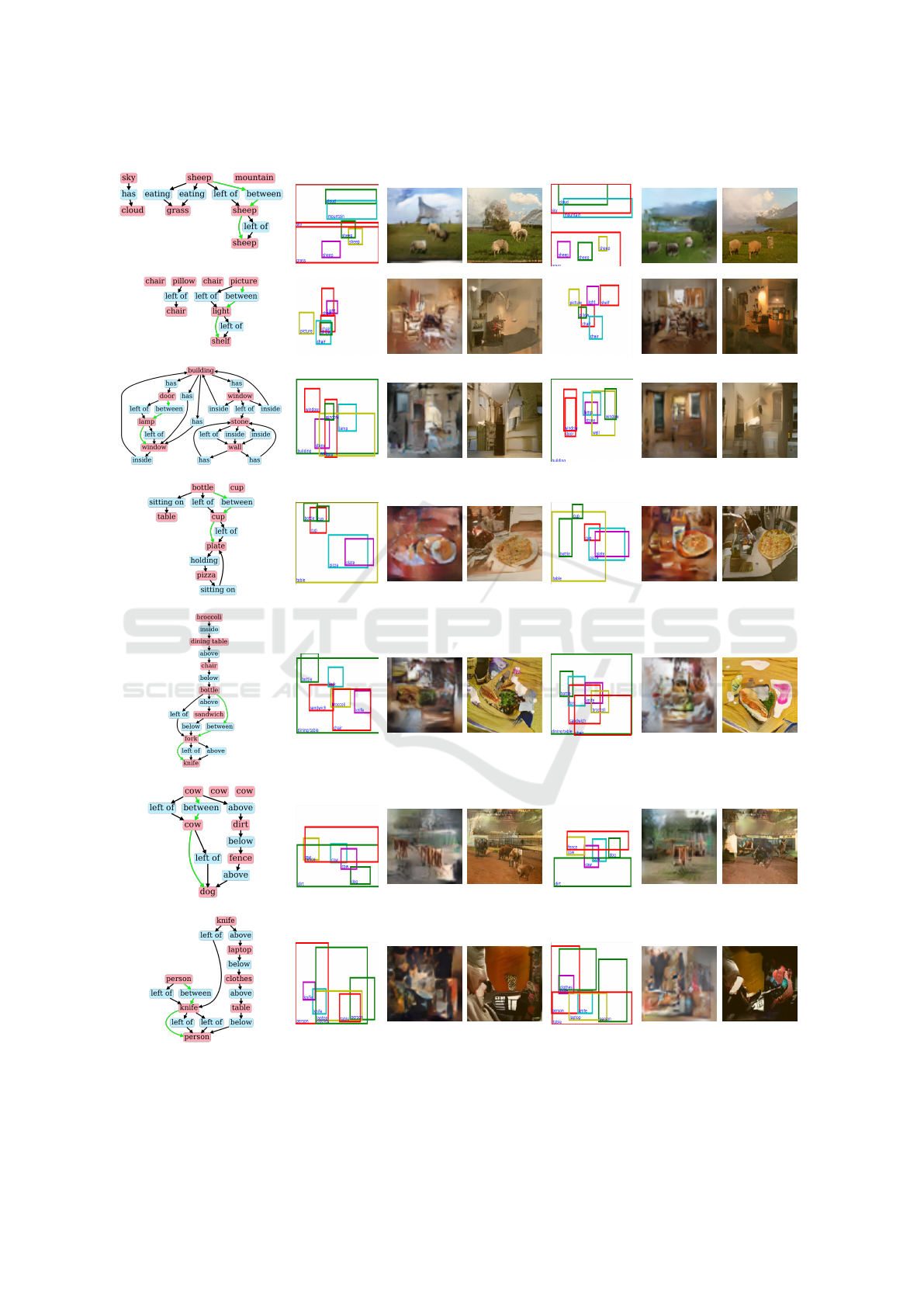
Next, we qualitatively evaluate the generated im-
ages. Figure 5 shows the generated images of hsg2im
and sg2im. The scene graph of the input to sg2im in
(a) has a path “sheep” (light blue bounding box) →
“left of” → “sheep” (yellow) → “left of” → “sheep”
(purple). However, we can confirm that “sheep” (yel-
low) is generated at a higher position than “sheep”
(light blue), and the “left of” relation is not satisfied.
On the other hand, in the layout generated by hsg2im,
three objects are generated in a positional relation
which satisfies the trinomial relation “sheep” (light
blue) → “between” → “sheep” (yellow) → “sheep”
(purple) in the hyper scene graph of the input. Also,
the scene graph of the input to sg2im in (b) has a
path “picture” (purple) → “left of” → “light” (light
blue) → “left of” → “shelf” (blue). However, “light”
and “shelf” bounding boxes are generated on top of
each other, and these objects are missing in the image
(with Layout2img). On the other hand, in the layout
generated by hsg2im, the bounding boxes for “light”
and “shelf” do not overlap each other, and these ob-
jects can be seen in the generated image (with Lay-
out2img). Thus, we can also confirm the effect of the
introduction of the trinomial hyperedge in the gener-
ated images.
6.4 Computational Time
We explain the computational time of the training and
the test phases in each of sg2im and hsg2im. We
used one GPU (NVIDIA TITAN RTX). From Table
4, we can confirm that there is no significant differ-
ence between sg2im and hsg2im in both the training
time and the test time. In some cases such as the train-
ing time in Visual Genome and COCO, hsg2im takes
longer time due to the addition of net3 in the proposed
model.
Table 4: Computational time of the training and the test
phases in each of sg2im and hsg2im.
Training Test
sg2im (COCO) 66.1h 127.6m
hsg2im (COCO) 66.4h 127.5m
sg2im (VG) 31.8h 196.1m
hsg2im (VG) 34.8h 191.5m
7 CONCLUSIONS
We have proposed an image generation model hsg2im
from a hyper scene graph. The proposed model is
an extension of the image generation model sg2im
(Johnson et al., 2018) from a scene graph with our ad-
dition of a hyperedge representing a trinomial relation
to the scene graph, in order to improve the positional
relations of the generated objects.
In the evaluation of the Positional relation of
Three Objects (PTO), the performance of hsg2im was
higher by about 12% and 20% on the 2017 COCO
Stuff (COCO) dataset and the Visual Genome dataset,
respectively, than sg2im. In the evaluation of the nat-
uralness of the generated images based on the Incep-
tion Score, the scores improved by about 0.25 for
VISAPP 2023 - 18th International Conference on Computer Vision Theory and Applications
192

(Hyper) Scene Graph
(a)
Layout
(sg2im)
sg2im wo
Layout2img
sg2im with
Layout2img
Layout
(hsg2im)
hg2im wo
Layout2img
hsg2im with
Layout2img
(b)
(c)
(d)
(e)
(f)
(g)
Figure 5: Comparison of images generated by sg2im (Johnson et al., 2018) and hsg2im. (a) ∼ (d) and (e) ∼ (g) are from the
Visual Genome and the MS COCO datasets, respectively. In the input for sg2im, the trinomial hyperedges “between” do not
exist.
Image Generation from a Hyper Scene Graph with Trinomial Hyperedges
193

the COCO dataset and by about 0.40 for the Visual
Genome dataset. In addition, we generated more nat-
ural images by using the layout-to-image model Lay-
out2img supplementally. Although we added only
“between” relation as a trinomial hyperedge, adding
other kinds of hyperedges would lead to generating
more consistent images with the input. Thus it is an
interesting direction for our future work.
REFERENCES
Agnese, J., Herrera, J., Tao, H., and Zhu, X. (2020). A Sur-
vey and Taxonomy of Adversarial Neural Networks
for Text-to-Image Synthesis. Wiley Interdisciplinary
Reviews: Data Mining and Knowledge Discovery,
10(4):e1345.
Caesar, H., Uijlings, J., and Ferrari, V. (2018). Coco-Stuff:
Thing and Stuff Classes in Context. In Proceedings of
the IEEE Conference on Computer Vision and Pattern
Recognition, pages 1209–1218.
Chen, Q. and Koltun, V. (2017). Photographic Image Syn-
thesis with Cascaded Refinement Networks. In Pro-
ceedings of the IEEE International Conference on
Computer Vision, pages 1511–1520.
Elgammal, A., Liu, B., Elhoseiny, M., and Mazzone, M.
(2017). CAN: Creative Adversarial Networks Gener-
ating “Art” by Learning About Styles and Deviating
from Style Norms. arXiv preprint arXiv:1706.07068.
Frolov, S., Hinz, T., Raue, F., Hees, J., and Dengel, A.
(2021). Adversarial Text-to-Image Synthesis: A re-
view. arXiv preprint arXiv:2101.09983.
Ghorbani, A., Natarajan, V., Coz, D., and Liu, Y. (2020).
DermGAN: Synthetic Generation of Clinical Skin Im-
ages with Pathology. In Machine Learning for Health
Workshop, pages 155–170. PMLR.
Goodfellow, I., Pouget-Abadie, J., Mirza, M., Xu, B.,
Warde-Farley, D., Ozair, S., Courville, A., and Ben-
gio, Y. (2014). Generative Adversarial Nets. Advances
in Neural Information Processing Systems, 27.
Gui, J., Sun, Z., Wen, Y., Tao, D., and Ye, J. (2021). A
Review on Generative Adversarial Networks: Algo-
rithms, Theory, and Applications. IEEE Transactions
on Knowledge and Data Engineering.
He, K., Zhang, X., Ren, S., and Sun, J. (2016). Deep Resid-
ual Learning for Image Recognition. In Proceedings
of the IEEE Conference on Computer Vision and Pat-
tern Recognition, pages 770–778.
He, S., Liao, W., Yang, M. Y., Yang, Y., Song, Y.-Z., Rosen-
hahn, B., and Xiang, T. (2021). Context-Aware Layout
to Image Generation with Enhanced Object Appear-
ance. In Proceedings of the IEEE/CVF Conference
on Computer Vision and Pattern Recognition, pages
15049–15058.
Heusel, M., Ramsauer, H., Unterthiner, T., Nessler, B., and
Hochreiter, S. (2017). GANs Trained by a Two Time-
Scale Update Rule Converge to a Local Nash Equilib-
rium. In NuerIPS.
Hinz, T., Heinrich, S., and Wermter, S. (2019). Generat-
ing Multiple Objects at Spatially Distinct Locations.
ArXiv, abs/1901.00686.
Hinz, T., Heinrich, S., and Wermter, S. (2022). Semantic
Object Accuracy for Generative Text-to-Image Syn-
thesis. IEEE Transactions on Pattern Analysis and
Machine Intelligence, 44:1552–1565.
Johnson, J., Gupta, A., and Fei-Fei, L. (2018). Image
Generation from Scene Graphs. In Proceedings of
the IEEE Conference on Computer Vision and Pattern
Recognition, pages 1219–1228.
Johnson, J., Krishna, R., Stark, M., Li, L.-J., Shamma, D.,
Bernstein, M., and Fei-Fei, L. (2015). Image Retrieval
Using Scene Graphs. In Proceedings of the IEEE Con-
ference on Computer Vision and Pattern Recognition,
pages 3668–3678.
Kingma, D. P. and Ba, J. (2015). Adam: A Method for
Stochastic Optimization. CoRR, abs/1412.6980.
Kingma, D. P. and Welling, M. (2013). Auto-Encoding
Variational Bayes. arXiv preprint arXiv:1312.6114.
Krishna, R., Zhu, Y., Groth, O., Johnson, J., Hata,
K., Kravitz, J., Chen, S., Kalantidis, Y., Li, L.-J.,
Shamma, D. A., et al. (2017). Visual Genome: Con-
necting Language and Vision Using Crowdsourced
Dense Image Annotations. International Journal of
Computer Vision, 123(1):32–73.
Li, Y., Ma, T., Bai, Y., Duan, N., Wei, S., and Wang,
X. (2019). PasteGAN: A Semi-Parametric Method
to Generate Image from Scene Graph. ArXiv,
abs/1905.01608.
Mirza, M. and Osindero, S. (2014). Conditional Generative
Adversarial Nets. arXiv preprint arXiv:1411.1784.
Mittal, G., Agrawal, S., Agarwal, A., Mehta, S., and Mar-
wah, T. (2019). Interactive Image Generation Using
Scene Graphs. ArXiv, abs/1905.03743.
Nie, D., Trullo, R., Lian, J., Petitjean, C., Ruan, S., Wang,
Q., and Shen, D. (2017). Medical Image Synthe-
sis with Context-Aware Generative Adversarial Net-
works. In International Conference on Medical Im-
age Computing and Computer-Assisted Intervention,
pages 417–425. Springer.
Odena, A., Olah, C., and Shlens, J. (2017). Conditional Im-
age Synthesis with Auxiliary Classifier GANs. In In-
ternational Conference on Machine Learning, pages
2642–2651. PMLR.
Radford, A., Metz, L., and Chintala, S. (2015). Un-
supervised Representation Learning with Deep Con-
volutional Generative Adversarial Networks. arXiv
preprint arXiv:1511.06434.
Reed, S. E., Akata, Z., Yan, X., Logeswaran, L., Schiele,
B., and Lee, H. (2016). Generative Adversarial Text
to Image Synthesis. ArXiv, abs/1605.05396.
Rezatofighi, H., Tsoi, N., Gwak, J., Sadeghian, A., Reid,
I., and Savarese, S. (2019). Generalized Intersection
over Union: A Metric and a Loss for Bounding Box
Regression. In Proceedings of the IEEE/CVF Con-
ference on Computer Vision and Pattern Recognition,
pages 658–666.
Russakovsky, O., Deng, J., Su, H., Krause, J., Satheesh, S.,
Ma, S., Huang, Z., Karpathy, A., Khosla, A., Bern-
VISAPP 2023 - 18th International Conference on Computer Vision Theory and Applications
194

stein, M., et al. (2015). ImageNet Large Scale Vi-
sual Recognition Challenge. International Journal of
Computer Vision, 115(3):211–252.
Salimans, T., Goodfellow, I., Zaremba, W., Cheung, V.,
Radford, A., and Chen, X. (2016). Improved Tech-
niques for Training GANs. Advances in Neural Infor-
mation Processing Systems, 29.
Schuster, S., Krishna, R., Chang, A., Fei-Fei, L., and Man-
ning, C. D. (2015). Generating Semantically Precise
Scene Graphs from Textual Descriptions for Improved
Image Retrieval. In Proceedings of the Fourth Work-
shop on Vision and Language, pages 70–80.
Sun, W. and Wu, T. (2019). Image Synthesis From Recon-
figurable Layout and Style . In Proceedings of the
IEEE/CVF International Conference on Computer Vi-
sion, pages 10531–10540.
Szegedy, C., Liu, W., Jia, Y., Sermanet, P., Reed, S.,
Anguelov, D., Erhan, D., Vanhoucke, V., and Rabi-
novich, A. (2015). Going Deeper with Convolutions.
In Proceedings of the IEEE Conference on Computer
Vision and Pattern Recognition, pages 1–9.
Van Den Oord, A., Kalchbrenner, N., and Kavukcuoglu, K.
(2016). Pixel Recurrent Neural Networks. In Interna-
tional Conference on Machine Learning, pages 1747–
1756. PMLR.
Vo, D. M. and Sugimoto, A. (2020). Visual-Relation Con-
scious Image Generation from Structured-Text. ArXiv,
abs/1908.01741.
Wu, X., Xu, K., and Hall, P. (2017). A Survey of Im-
age Synthesis and Editing with Generative Adver-
sarial Networks. Tsinghua Science and Technology,
22(6):660–674.
Zhang, H., Xu, T., Li, H., Zhang, S., Wang, X., Huang,
X., and Metaxas, D. N. (2017). StackGAN: Text to
Photo-Realistic Image Synthesis with Stacked Gen-
erative Adversarial Networks. In Proceedings of the
IEEE International Conference on Computer Vision,
pages 5907–5915.
Zhang, H., Xu, T., Li, H., Zhang, S., Wang, X., Huang, X.,
and Metaxas, D. N. (2018). Stackgan++: Realistic
Image Synthesis with Stacked Generative Adversarial
Networks. IEEE Transactions on Pattern Analysis and
Machine Intelligence, 41(8):1947–1962.
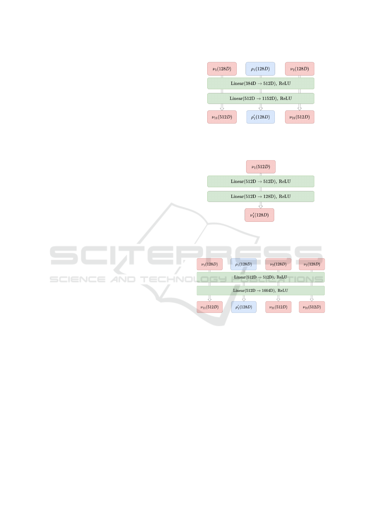
APPENDIX
We show the detailed structure of hg2sim. Fig. 6,7,
and 8 are net1, net2 and net3, which are used in the
(hyper) graph convolutional network, respectively.
Figure 6: Structure of net1. It receives two 128-dimensional
object vectors and one relation vector corresponding to e ∈
E, and outputs two 512-dimensional object vectors and one
128-dimensional relation vector.
Figure 7: Structure of net2. It receives one 512-dimensional
object vector, which is the output of net1 and net3, and out-
puts a 128-dimensional object vector by conducting dimen-
sionality reduction.
Figure 8: Structure of net3. It receives three 128-
dimensional object vectors and one relation vector corre-
sponding to q ∈ Q, and outputs three 512-dimensional ob-
ject vectors and one 128-dimensional relation vector.
Image Generation from a Hyper Scene Graph with Trinomial Hyperedges
195