Exotic Bets: Evolutionary Computing Coupled with Bet Mechanisms for
Model Selection
Simon Reichhuber
a
and Sven Tomforde
b
Intelligent Systems, Kiel University, Hermann-Rodewald-Str. 3, 24118 Kiel, Germany
Keywords:
Evolutionary Algorithms, Bet-Based Learning, Model Selection, Gradient-Free Optimisation.
Abstract:
This paper presents a framework for the application of an external bet-based evolutionary algorithm to the
problem of model selection. In particular, we have defined two new risk functions, called sample space exotic-
ness and configuration space exoticness. The latter is used to manage the risk of bet placement. Further, we
explain how to implement the bet-based approach for model selection in the domain of multi-class classifica-
tion and experimentally compare the performance of the algorithm to reference derivative-free hyperparameter
optimisers (GA and Bayesian Optimisation) on MNIST. Finally, we experimentally show that for the classifiers
SVM, MLP, and Nearest Neighbors the balanced accuracy can be increased by up to three percentage points.
1 INTRODUCTION
The field of Evolutionary Algorithms (EAs) has in-
tensively been expanded throughout the last decades.
Similar to other nature-inspired algorithms such as
Neural Networks, the design of these algorithms fol-
lowed a bottom-up approach, where only the main
ideas from nature have been simulated: In Neu-
ral Networks the neural structure or in EAs the en-
coding scheme for bits of information as chromo-
somes. With the increasing computing capabilities,
researchers have extended the basic concept of EAs to
solve more complex problems, evolving these meth-
ods to one of the standard methods for non-gradient-
based optimisation.
At the same time, the underlying methodology of
EAs remained the same: The solution of the opti-
misation problem is evolved by a randomly gener-
ated population with the help of the operator’s se-
lection, recombination and mutation successively ap-
plied over several generations to form a ”fitter” popu-
lation. The term ”fitness” indicates how close a chro-
mosome from the population has come to the opti-
mum of the optimisation problem.
Since the idea of ”finding the fittest” of a large
population is also well-known in the domain of bet-
ting, we proposed to augment the concept of the basic
EA by introducing another population, the so-called
a
https://orcid.org/0000-0001-8951-8962
b
https://orcid.org/0000-0002-5825-8915
”bet population” (Reichhuber and Tomforde, 2021;
Reichhuber and Tomforde, 2022). Both populations
are evolved like normal EAs, but the bet population
consists of individuals that have insight into the solu-
tion space. With this, they can place bets (here repre-
sented as Gaussians) to all individuals that are located
in the vicinity of the bet position. These individuals
benefit from the bets by increasing their fitness. On
the other hand, a bet individual can win or lose de-
pending on whether the fitness of the individuals in
the vicinity of the bet location has increased or de-
creased from the last generation.
In this paper, we extend and refine the idea and
adapt the concept to the model selection problem. The
underlying concept is that this adaptation tackles two
major problems of EAs: First, the diversity of the
fitness of the population stays healthy, meaning the
trade-off between exploring weak solutions and ex-
ploiting and refining the so-far best solutions. Second,
also the diversity of the locations of the solutions is
increased, which is especially interesting for solving
optimisation problems with multiple local optima, as
is the case in model selection.
For the evaluation of the novel approach, we have
chosen the field of model selection for multi-class
classification and compared our approach to other
model selection algorithms, such as standard Genetic
Algorithms (GAs) or Bayesian Optimisation (BO).
We propose two novel exoticness metrics that are used
for risk management of the betting process and show
experimentally the resulting behaviour.
Reichhuber, S. and Tomforde, S.
Exotic Bets: Evolutionary Computing Coupled with Bet Mechanisms for Model Selection.
DOI: 10.5220/0011698500003393
In Proceedings of the 15th International Conference on Agents and Artificial Intelligence (ICAART 2023) - Volume 2, pages 259-267
ISBN: 978-989-758-623-1; ISSN: 2184-433X
Copyright
c
 2023 by SCITEPRESS – Science and Technology Publications, Lda. Under CC license (CC BY-NC-ND 4.0)
259

The remainder of the paper is organised as fol-
lows. Section 2 discusses related work in the area
of Model Selection based on evolutionary algorithms,
also covering preliminary work on bet-based evolu-
tionary algorithms. Section 3 explains our approach
and Section 4 evaluates the methodology in compari-
son to other approaches with the goal to evolve suit-
able hyperparameters
1
for classifiers. Finally, Sec-
tion 5 summarises the paper and gives an outlook to
future work.
2 RELATED WORK
In the year 1988 Peter Asch and Richard Quandt anal-
ysed empirical data consisting of horse racetrack bets
and found some interesting results (Asch and Quandt,
1988). In the scenario, they found evidence that the
total of all bets resulting from individual win proba-
bility estimations are good approximates for the ob-
jective win probabilities. The winning probability of
a single horse has no Markov property in that sense
that even if its last run was not successful, it may not
have met its win conditions, but normally it is a hid-
den champion. The trust in such hidden champions
may result in so called long-shot bets that require the
perseverance to lose money over multiple unsuccess-
ful bet placements. The authors found tendencies that
a betting bias exists in that favourites are underbet and
long-shots overbet. These findings may have inspired
the authors to the title ’Exotic’ bets. The emergent
effect of approximating the win probabilities by the
sum of the subjective bets of different betting agents
inspired us to simulate the process of betting. For
the sake of generality, we replaced the horse riding
scenario with an evolutionary environment of an arbi-
trary fitness function, which shall be optimised (Re-
ichhuber and Tomforde, 2021). In this paper, we fo-
cus on Model Selection in the scenario of classifica-
tion, which is based on the architecture of a Genetic
Algorithm (GA).
John Holland published his idea of implementing
GAs and refined it to a large extent (Holland, 1975;
Booker et al., 1989). Afterwards, several extensions
have been proposed. Inspired by evolution, the ba-
sic idea was to develop a natural selection process
through selection, recombination and mutation. Af-
ter a certain number of generations, the procedure al-
lowed to create individuals, which are better adapted
to the environment.
1
The terms hyperparameter and model are used synony-
mously in this paper. The same holds for hyperparameter
optimisation and model selection.
The adaptations of GAs to real numbers and
modifications of different mutation or recombination
strategies reducing the number of generations, hence
the number of fitness function calls, turned the al-
gorithm into a general-purpose optimisation tool for
derivative-free multi-variate optimisation. Therefore,
many scientists in the domain of Machine Learning
(ML) made suggestions on how to adapt GAs to the
task of model selection. Another question was to
which environments the GAs are applicable to if sci-
entists think about the model selection task in Ma-
chine Learning.
In the literature, one can find multiple applica-
tions of GAs applied to Model Selection. For ex-
ample, (Guerbai et al., 2022) have applied one-class
support vector machines in the scenario of Novelty
Detection and multi-class classification or (Buchtala
et al., 2005) evolved radial basis function classifiers
for data mining applications. Furthermore, the au-
thors of (Young et al., 2015) applied EAs to deep neu-
ral networks with multiple convolutional and fully-
connected layers. Similar to our approach, in (de Lac-
erda et al., 2002) the authors used bootstrapping for
modelling the true prediction error but besides this
paper, most of the architectures rely on the basic GA
as it is presented by Holland (Holland, 1975). How-
ever, there are multiple suggested architectures such
as the Island/Course-grained Model as it is described
in (Gong et al., 2015) or the cellular distributed EAs,
which are analysed in (Giacobini et al., 2003; Gi-
acobini et al., 2004) – for example regarding their
takeover times, which is the duration that allows a
dominant individual to occupy the whole population.
There have also been other types of EAs, besides
the encoding of individuals. For example, Thomas
B
¨
ack (B
¨
ack and Schwefel, 1993) categorised three
types of EAs: Evolution Strategies, Evolutionary Pro-
gramming, and Genetic Algorithms (Forrest, 1996;
Grefenstette, 1993; Bies et al., 2006; Paterlini and
Minerva, 2010; Lessmann et al., 2006; Devos et al.,
2014; de Lacerda et al., 2002). First bet mechanics
have been applied to EAs in the context of a bet mech-
anism, where an external bet population coexists and
is able to place bets on the main population (Reichhu-
ber and Tomforde, 2021; Reichhuber and Tomforde,
2022). Each individual in the bet population repre-
sents a certain bet strategy and places bets on the main
population. These bets directly influence the fitness of
the main population for the sake of high diversity.
Betting is not the only methodology, which steers
the evolution of GAs from an external source. In
(Guerbai et al., 2022), for instance, the evolutionary
process is steered with the help of temperature-based
control. Here, the EAs are used to optimise parame-
ICAART 2023 - 15th International Conference on Agents and Artificial Intelligence
260

ters of radial basis networks for novelty detection and
multi-class classification (Frazier, 2018; Snoek et al.,
2012; Shahriari et al., 2015; Bodnar et al., 2020).
3 METHODOLOGY
In the following, we describe the methodology of
model selection for classification with the means
of bet-based evolutionary algorithms. Mathemati-
cally, we solve an optimisation problem (see Equa-
tion 1), in which we want to find the optimal hy-
perparameter θ
∗
∈ Θ among a predefined set of hy-
perparameters Θ used to train a multi-class classifier
f
θ,X
train
,Y
train
: X → Y , which has been trained on the
training data (X
train
,Y
train
).
Furthermore, a test error function is given
test-error : X × Y × Y → R measuring the classi-
fication error, i.e. a quantification of the difference
between the true labels Y
test
and the predicted labels
f
θ
(X
test
) ∈ Y . With these ingredients, we can define
the optimisation problem:
θ
∗
= argmin
θ∈Θ
test-error(X
test
,Y
test
,
f
θ,X
train
,Y
train
(X
test
)).
(1)
Due to the size of the parameter space and the com-
putational complexity of the test error, we iteratively
find a near-to-optimal solution given a limited com-
putation time. After a rough description of the basic
procedure, the novel genetic operators are explained
in detail. These are Initialisation, Encoding, and fit-
ness calculation. At the end of the section, we de-
scribe the bet placement mechanism and explain the
two exoticness metrics used for risk management of
betting.
3.1 Procedure of External Bet-Based
Evolutionary Algorithms for Model
Selection
Finding the optimal D hyperparameters as the opti-
mal hyperparameter configuration θ
∗
∈ R
D
of Equa-
tion 1, we establish a bet-based Evolutionary Algo-
rithm (BEA). By that, we refer to the minimisation
of the test error of a machine learning model through
evolutionary algorithms steered by an external popu-
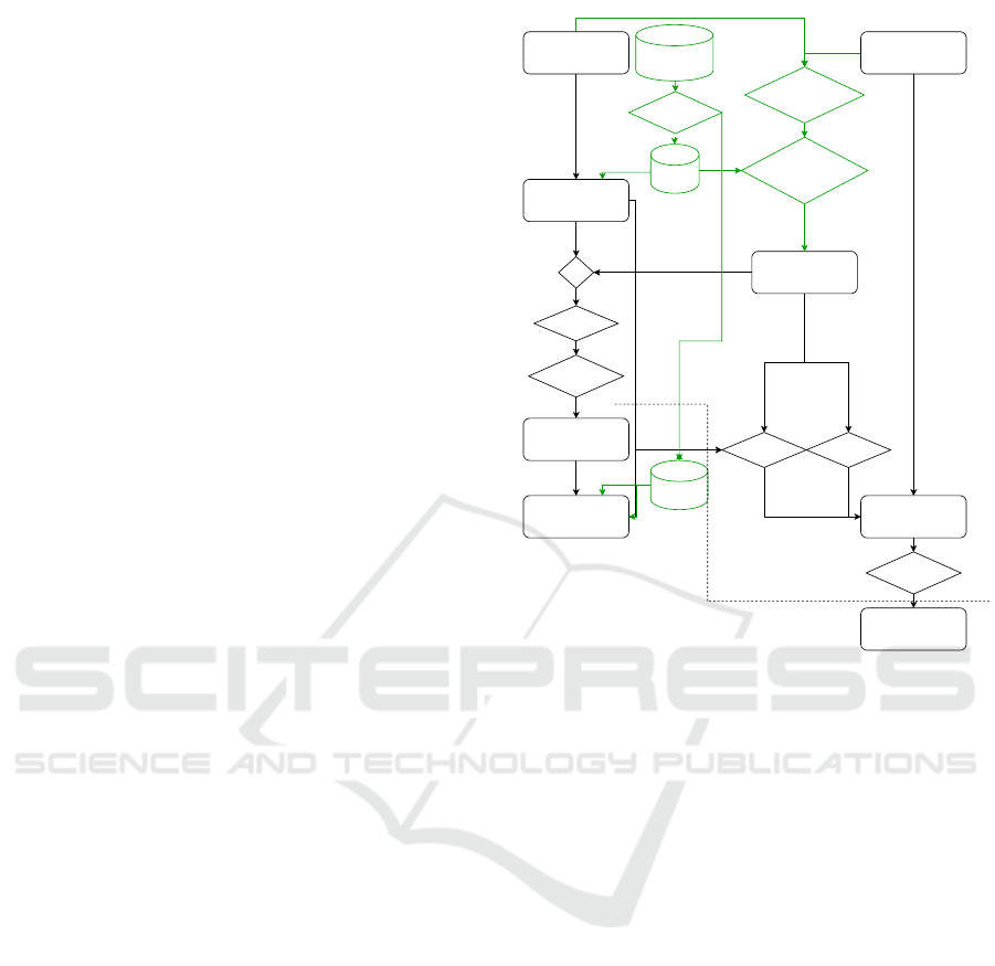
lation. In Figure 1, the basic idea of the two coexisting
populations and their interaction during two iterations
is visualised. The separation of both populations is
taken from (Reichhuber and Tomforde, 2022) with a
few adaptations (highlighted in green in Figure 1).
Main Population
Fitness
Bet Population
+
Next Main
Population
Winnings
test-error
Bets
Next test-error Fitness
GA Operations
Next Bet Population
GA Operations
Losses
Training Data
Bootstrapping
Next
Subset
Subset
Compute
Configuraiton Space
Exoticness
Compute Sample
Set Exoticness
1. Iteration
2. Iteration
Figure 1: External bet-based Evolutionary Algorithm pro-
cedure applied to Model Selection task.
In the first iteration, a population is initialised,
which we denote the main population P
main
. Ad-
ditionally, we create the coexisting population de-
noted bet population P
bet
. Both populations are
uniform-randomly drawn from the hyperparameter
ranges, θ
θ
θ
min
, θ
θ
θ
max
∈ R
D
and the sigma step ranges
σ
σ
σ
max
, σ
σ
σ
max
∈ R
D
are given a-priori. Afterwards, a
new, small subset (X
b
,Y
b
) is drawn from the training
data (X
train
,Y
train
), which we call bootstrapped set.
Then, each individual of the main population is eval-
uated according to the test error measuring the differ-
ence between the test data X
test
,Y
test
and the predic-
tions from a trained classifier. The latter is equipped
with parameters from the individual and was trained
on the bootstrapped set.
Extracting the risk of the current bet-placement,
which we explain later, each individual j = 1, . . . , N
bet
of the bet population places bets on the parameter
space represented by a Gaussian with diagonal co-
variance, i.e. N (x
x
x|µ
µ
µ
j
, σ
σ
σ
j
), µ
µ
µ
j
, σ
σ
σ
j
∈ R
D
. Individuals
of the main population benefit from a fitness increase
when they are located in the vicinity of bets of the
main population. The exact calculation can be seen in
Algorithm 1.
Exotic Bets: Evolutionary Computing Coupled with Bet Mechanisms for Model Selection
261

Algorithm 1: Procedure of exotic bet-based model selec-
tion.
1: function EXOTIC BET-BASED MODEL SELEC-
TION( f , θ
θ
θ
min
, θ
θ
θ
max
, σ
σ
σ
min
, σ
σ
σ
max
,
X
train
,Y
train
, X
test
,Y
test
)
 Normalise the data
2: X
X
X
train
← norm(X
X
X
train
, µ
train
, σ
train
)
3: X
X
X
test
← norm(X
X
X
test
, µ
train
, σ
train
)
 Initialise main and bet population
4: P
(0)
main
← {x
x
x
i
= (x
i,d
)
D
d=1
)}
N
main
i=1
,
5: x
i,d
∼ U([θ
min,d
, θ
max,d
])
6: P
(0)
bet
← {b
b
b
j
= (µ
j,d
, σ
j,d
)}
N
bet
j=1
,
7: µ
j,d
∼ U([θ
min,d
, θ
max,d
])
8: σ
j,d
∼ U([σ
min,d
, σ
max,d
])
9: for each g = 1, . . . , #Generations do
 Draw new bootstrap subset
10: X
b
,Y
b
← draw(X
train
,Y
train
)
 Calculate Sample Space Exoticness
11: SSE ← 1 − LDOVL(X
train
, X
b
)
12: for each i = 1, . . . , N
main
do
 Calculate fitness of main population
13: F
main,i
←
14: −test-error
15: (X
test
,Y
test
, f
x
x
x
i
,X
b
,Y
b
(X
test
))
 Calc. Configuration Space Exoticness
16: CSE
i
← CSE = 1 − N (x
x
x|P
main
)
 Calculate the individual risk
17: risk
i
← (1 − SSE) ∗CSE
i
 Calculate bets
18: bet
i
← risk
i
∗
1
N
bet
∑
N
bet
j
N (x
x
x
i
|µ
µ
µ
j
, σ
σ
σ
j
)
 Add individual bet to the fitness
19: F
main,i
← F
main,i
+ bet influence
20: ∗ bet
i
21: end for
22: for each j = 1, . . . , N
bet
do
 Calculate fitness of bet population
23: F
bet, j
←
1
N
main
∑
N
main
i=1
N (x
x
x
i
|µ
µ
µ
j
, σ
σ
σ
j
)
24: end for
 Apply GA Operations:
 Selection, Recombination, Mutation
25: P
(g)
main
← GA-Operation(P
(g−1)
main
, F
main
)
26: P
(g)
bet
← GA-Operation(P
(g−1)
bet
, F
bet
)
27: end for
28: θ
θ
θ
∗
←
argmax
x
x
x∈P
(g)
main
29: −test-error(X
test
,Y
test
,
30: f
x
x
x
i
,X
train
,Y
train
(X
test
))
31: return θ
θ
θ
∗
32: end function
To calculate the risk of betting, the bootstrapped
subset is analysed by each individual of the bet pop-
ulation to estimate an individual value of exoticness
called Sample Space Exoticness. Additionally, given
the deviation of the bet individual’s own guess to all
other guesses, (also known as Configuration Space
Exoticness), each bet individual is able to calculate
its own risk of the bet placement as follows:
bet
i
= risk
i
∗
1
N
bet
N
bet
∑
j
N (x
x
x
i
|µ
µ
µ
j
, σ
σ
σ
j
) (2)
where the risk is a combination of SSE and CSE:
risk
i
= (1 − SSE) ∗CSE
i
. (3)
The calculated bets will then be added to the main
population’s fitness. After this correctly predicted
wins or losses of fitness in the main population are
used as fitness for the bet population. After the eval-
uation of the fitness of both populations, the Genetic
Operations will be applied, which are listed below and
explained in the following.
1) Selection of the parents for example by using uni-
versal stochastic sampling
2) Recombination of the parents to obtain the chil-
dren population called offspring, e.g. with the
help of uniform crossover
3) Mutations on all individuals beside a small frac-
tion representing the elite individuals, e.g. with
one-step mutations
4) Declare the parental population and the offspring
as next generation
3.2 Genetic Operators
In the following, we point out the differences between
our approach compared to the EA presented in (Re-
ichhuber and Tomforde, 2021). Following the general
procedure of an EA, we describe each step in detail:
3.2.1 Initialisation
In the first step, the individuals of both populations
are uniformly drawn from the configuration space
x
x
x
i
∼U[x
x
x
min
, x
x
x
max
] ⊂ R
D
. Here, the limits of the hyper-
parameters have to be defined in advance. Extensions
to a dynamically increasing feature space are possible
but have not been considered further in this paper.
3.2.2 Encoding
In the main population, each individual represents
a specific hyperparameter configuration. Depending
on the classifier we have to choose from, which re-
quires D hyperparameters, we encode the individual
ICAART 2023 - 15th International Conference on Agents and Artificial Intelligence
262

Main Population
Bet Population
Population










…
…







parents








…

  



children



…



…


individuals
Configuration Space
…













…
…








parents












…



 




children



…



…
…
 individuals
Sample Space
Figure 2: Encoding and interactions of the main population
and the bet population.
i ∈ {1, . . . , N
main
} of the main population of size N
main
as:
x
x
x
i
= (x
x
x
i
[1], . . . , x
x
x
i
[D])
On the other hand, we encode the individual of the bet
population j ∈ N
bet
such that each bet individual con-
sists of two components: The estimated guess of the
optimum µ
µ
µ ∈ R
D
and the certainty about this guess
σ
σ
σ ∈ R
D
. Equipped with these parameters, the bet in-
dividual is able to calculate a so-called sample space
exoticness (SSE) and configuration space exoticness
(CSE), which are explained in more detail in Sec-
tion 3.3.
In Figure 2, the encoding and interactions of both
populations are depicted. The bet-based parameters
are abbreviated as:
b
b
b
j
= (b
b
b
j
[1], . . . , b
b
b
j
[2D])
3.2.3 Fitness Calculation: Main Population
The fitness function aims at an estimation of the test
classification balanced accuracy of the classification
problem. For most of the models, it is computation-
ally infeasible to train and test each individual on the
whole given sample data, i.e. the matrix inversion
in finding the optimal hyperplane in support vector
machines has time complexity O(n
3
) and cannot deal
with magnitudes of millions. Therefore, we test each
individual on a small subset. The problem of ap-
proximating the test error from a small subset was
pointed out by (Lessmann et al., 2006). They argue
that the problem of finding the correct hyperparame-
ter for support vector machines is quite hard when no
validation set is available. To make the most out of the
subset, we use k-fold cross-validation as in (de Lac-
erda et al., 2002). Each individual’s hyperparameter
choice is evaluated on a small subset of the training
data, which is uniformly and randomly drawn with
replacement. The training data represents a standard
classification problem consisting of N measurements
x
i
∈ X and their target values y
i
∈ Y . In the case of
classification, we suggest the balanced accuracy value
as a validation metric.
Since the computing time for the fitness calcula-
tion crucially influences the total computing time (the
fitness has to be calculated in each iteration for each
individual), we consider the balanced accuracy on a
bootstrapped set as a computational low-cost estima-
tion of the test error. Since the calculation of the fit-
ness value has a sensitive share in the total computing
time of the algorithm, it should take as little time as
possible. To avoid overfitting to a specific bootstrap
set, we repeatedly draw a novel set in each iteration.
Using bootstrapping we draw N
b
<< N
train
samples
from the training data. These evaluate the balanced
accuracy score for each configuration. In addition to
the negative test error the fitness is refined by the bets:
F
main,i
← F
main,i
+ bet influence ∗ bet
i
, (4)
where bet influence ∈ R
+
0
is a parameter that con-
trols the intensity of betting.
3.2.4 Fitness Calculation: Bet Population
The fitness of the bet population is then defined as:
F
bet
(b
b
b
j
) =
1
N
main
N
main
∑
i=1
N (x
x
x
i
|µ
µ
µ
j
, σ
σ
σ
j
) (5)
3.3 Sample Space Exoticness and
Configuration Space Exoticness
Each bet individual places bets according to risk man-
agement based on the Configuration Space Exoticness
and the Sample Space Exoticness. The Configuration
Space Exoticness expresses the deviation of a hyper-
parameter from the main population and the Sample
Space Exoticness is referred to the deviation of the
bootstrapped set to the training set.
3.3.1 Configuration Space Exoticness
Based on the hyperparameter configuration x
x
x
i
, repre-
sented by an individual of the main population, the bet
individual calculates the Configuration Space Exotic-
ness (CSE) value for each sample. This value repre-
sents the deviation of the hyperparameter to all other
hyperparameters of the main population and is mea-
sured as the normal distribution, which can be seen in
Equation 6
CSE = 1−N (x
x
x|P
main
) = 1−N (x
x
x|µ
µ
µ
P
main
, σ
σ
σ
P
main
) (6)
, where means and variances of the main population
are defined as follows:
µ
µ
µ
P
main
=
1
N
main
∑
x
x
x∈P
main
x
x
x,
Exotic Bets: Evolutionary Computing Coupled with Bet Mechanisms for Model Selection
263

σ
σ
σ
P
main
=
1
P
main
∑
x
x
x∈P
main
(x
x
x − µ
µ
µ
P
main
)
2
.
3.3.2 Sample Space Exoticness
On the other hand, for each bootstrapped subset X
b
drawn at the beginning of a generation, a bet individ-
ual can calculate its Sample Space Exoticness value
SSE(X
b
) as seen in Equation 7.
SSE(X
(t)
) = 1 − LDOVL(X
train
, X
b
) (7)
The function LDOVL is a special metric for the compar-
ison of two distributions, which we designed for the
requirements of exotic BEAs. When calculating the
similarity of distributions in the configuration space, a
major problem arises: On the one hand, hyperparam-
eters can be sensitive to slight changes, on the other
hand, local maxima can be far from each other. This
means that the similarity measure has to be sensible
to overlapping Gaussians in the vicinity of each other
(like it holds for the joint probability or the overlap-
ping coefficient (OVL) (Inman and Jr, 1989) ) and
simultaneously has to be capable of measuring far-
distant Gaussians (like the Euclidean distance of the
means or the RMSE of the means and the standard de-
viations) without the risk of vanishing similarity due
to numerical instabilities.
Therefore, we have developed a so-called long-
distant overlapping coefficient (LDOVL).
LDOVL. To measure slight differences of two dis-
tributions, which we assume in the case of bootstrap-
ping, we base our approach on the overlapping coeffi-
cient (OVL) (Inman and Jr, 1989). Given two normal
distributions N (·|µ
1
, σ
1
) and N (x|µ
2
, σ
2
) the over-
lapping coefficient is calculated as following:
OV L(µ
1
, σ
1
, µ
2
, σ
2
) =
Z
∞
−∞
min(N (x|µ
1
, σ
1
), N (x|µ
2
, σ
2
))dx.
(8)
One drawback of the OVL is that it vanishes for long-
distant distributions, where |µ
1
− µ
2
| >> σ
1
+ σ
2
. To
get around this problem, we introduce two areas: The
touching area and the long-distant area. The touch-
ing area is defined for distributions where |µ
1
− µ
2
| ≤
k(σ
1
+σ
2
) with k is a multiplier for the standard devi-
ations. Within this range, we refer to touching distri-
butions and derive a normalised version of the over-
lapping coefficient that is not vanishingly small. The
normalised version of the OVL is derived as follows:
OV L
0
(µ
1
, σ
1
, µ
2
, σ
2
) =
OV L(µ
1
, σ
1
, µ
2
OV L
min
(σ
1
, σ
2
)
OV L
max
(σ
1
, σ
2
) − OV L
min
(σ
1
, σ
2
)
(9)
where OV L
min
(σ
1
, σ
2
) =
OV L(0, σ
1
, 0 + k ∗ (σ
1
+ σ
2
), σ
2
)
and OV L
max
(σ
1
, σ
2
) =
OV L(0, σ
1
, 0, σ
2
)
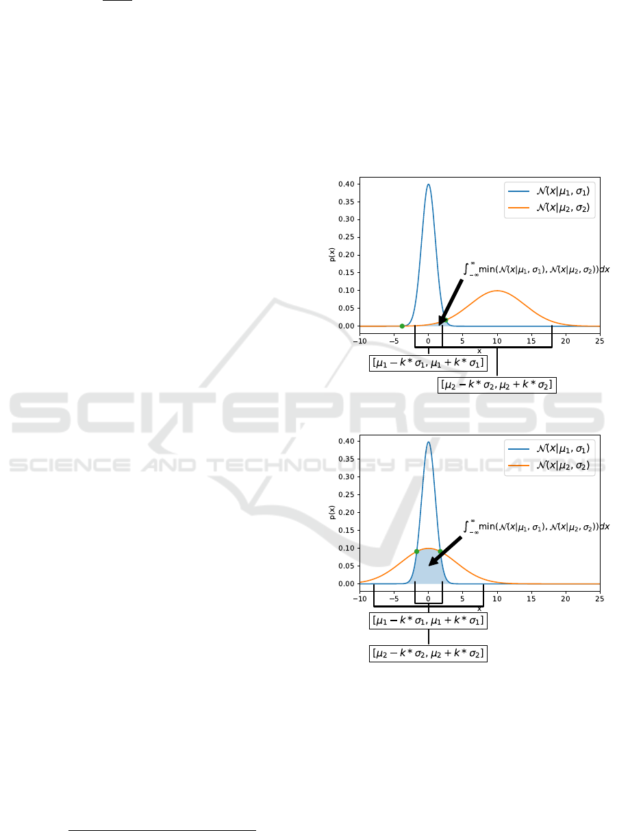
In the formula above, we take the min-max nor-
malisation based on the minimum OVL value (cf. Fig-
ure 3a) and the maximum OVL value (cf. Figure 3b)
that is possible when shifting the second distribution
over the other without changing the standard devia-
tions.
(a) Minimum overlapping.
(b) Maximum overlapping.
Figure 3.
In contrast to the touching area, the long-distant
area is only used for long-distant distributions, where
|µ
1
− µ
2
| > k ∗ (σ
1
+ σ
2
). Here, we use the propor-
tion of the distance of both means |µ
1
− µ
2
| to the
maximum feature range f
max
− f
min
and normalise this
value with the min/max normalisation.
ICAART 2023 - 15th International Conference on Agents and Artificial Intelligence
264

Figure 4: Long-distant-overlapping coefficient (LDOVL)
of two Normal distributions N (µ
1
= 0, σ
1
= 1) and
N (µ
2
, σ
2
= 4), µ
2
∈ [−40, 40]. Maximum LDOVL-value
is observed where the means of the two distributions are
equal, i.e. µ
1
= µ
2
= 0.
LD
0
(µ
1
, σ
1
, µ
2
, σ
2
) = 1 −
|µ
1
− µ
2
| − k ∗ (σ
1
+ σ
2
)
f
max
− f
min
− k ∗ (σ
1
+ σ
2
)
(10)
Finally, to take care of a given feature range de-
fined within a minimum/maximum feature value, i.e.
[ f
min
, f
max
], we cap distances, where one distribution
is outside the feature range to zero.
Combining all cases into one formula and intro-
ducing a weight to shift between the proportion of
touch distance and long-distance, we summarise the
long distant overlapping coefficient (LDOVL):
LDOV L(µ
1
, σ
1
, µ
2
, σ
2
) =





0 if I holds
(1 − λ) + λ ∗ OV L
0
(µ
1
, σ
1
, µ
2
, σ
2
), if II holds
(1 − λ) ∗ LD
0
(µ
1
, σ
1
, µ
2
, σ
2
), if III holds
,
where
I : µ
1
6∈ [ f
min
, f
max
] or µ
2
6∈ [ f
min
, f
max
]
II : |µ
1
− µ
2
| ≤ k ∗ (σ
1
+ σ
2
)
III : k ∗ (σ
1
+ σ
2
) < |µ
1
− µ
2
| ≤ f
max
− f
min
and 0 ≤ λ ≤ 1
(11)
For a better understanding, we plotted the dif-
ferent LDOVL values of two distributions (see Fig-
ure 4). Here, the first distribution remains constant
(N (µ
1
= 0, σ
1
= 1)) and the mean value of the sec-
ond distribution is shifted over the range -40 to 40
(N (µ
2
, σ
2
= 4)). We set the standard deviation mul-
tiplier to 2, which means that the touching area is de-
fined between −k ∗ (σ
1
+ σ
2
) = −2 ∗ (1 + 4) = −10
and +k ∗ (σ
1
+ σ
2
) = 2 ∗ (1 + 4) = 10.
One-Dimensional Box Embedding. As the metric
LDOVL is only applicable for one dimensional point
Figure 5: One-dimensional box embedding.
Table 1: Hyperparameter ranges for polynomial support
vector machines (Poly SVM), radial basis function sup-
port vector machines (RBF SVM), multi-layer perceptrons
(MLP), and nearest neighbours (NN). The Poly SVM is
equipped with the kernel k(x
x
x, x
x
x
0
) = (γhx
x
x, x
x
x
0
+ ri)
d
and the
RBF SVM with the kernel k(x
x
x, x
x
x
0
) = exp(−γ||x
x
x − x
x
x
0
||
2
).
Classifier Hyperparameters Parameter grid
Poly SVM
C Log([e − 3, e3])
r U([0, 100])
d [1, . . ., 6]
γ Log([e − 3, e3])
RBF SVM
C Log([−3, 3])
d [1, . . ., 4]
γ Log([e − 3, e3])
pca comp [5, .. . , 200]
MLP
layers
{(300), (150, 150), (100,200), (200, 100),
(100, 100, 100), (75,75, 75, 75),
(50, 100, 100, 50),(100, 50, 50, 100)}
α Log([e − 6, e − 1])
batch size {2
1
, 2
2
, . . . , 2
6
}
learning rate {
0
constant
0
,
0
adaptive
0
}
learning rate init Log([e − 4, e − 1])
activation f unction {
0
identity
0
,
0
logistic
0
,
0
tanh
0
,
0
relu
0
}
NN
# neighbours [1, 2, 3]
weights [
0
uniform
0
,
0
distance
0
]
p-norm U[1, 3]
distributions, we applied a one-dimensional box em-
bedding as visualised in Figure 5.
4 EXPERIMENTAL EVALUATION
We conducted a showcase on the dataset mnist (see
Table 2) of using exotic bet-based Evolutionary Al-
gorithms (exotic BEA) for the hyperparameter opti-
misation using the classifier from Table 1 with their
most important parameters and selected a hyperpa-
rameter range with specific scale. The classifiers are
taken from the python library sklearn (version 1.1.1).
All classifiers besides NN are preceded by a nor-
malisation consisting of a zero-mean-unit-standard-
deviation transformation and a min-max scaling to the
range [−1, 1].
Table 2: Properties of used dataset mnist.
Dataset # Features (train size, test size)
mnist (LeCun et al., 2010) (28, 28) gray images (60k, 10k)
Exotic Bets: Evolutionary Computing Coupled with Bet Mechanisms for Model Selection
265

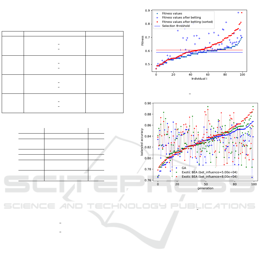
Table 3: Hyperparameter Optimisation (HPO) comparison
of the algorithms Genetic Algorithms (GA), Exotic bet-based
Evolutionary algorithms Exotic BEA, and Bayesian Opti-
misation (BO) on the mnist dataset.
Classifier HPO balanced accuracy
Poly SVM
GA 0.864
Exotic BEA (bet infl. = 5e4) 0.898
Exotic BEA (bet infl. = 8e4) 0.889
Bayesian Optimisation 0.844
RBF SVM
GA 0.925
Exotic BEA (bet infl. = 5e4) 0.948
Exotic BEA (bet infl. = 8e4) 0.925
Bayesian Optimisation 0.902
NN
GA 0.910
Exotic BEA (bet infl. = 5e4) 0.904
Exotic BEA (bet infl. = 8e4) 0.931
Bayesian Optimisation 0.901
MLP
GA 0.903
Exotic BEA (bet infl. = 5e4) 0.922
Exotic BEA (bet infl. = 8e4) 0.945
Bayesian Optimisation 0.892
Table 4: Parameters used for the evolutionary algorithm.
Parameter Description Value
N
P
Population size 100
N
G
Number of genera-
tions
100
r
p
Parents ratio 50 %
r
e
Elites ratio 1 %
p
µ
µ
µ
Mutation probability
for means
1 %
p
σ
σ
σ
Mutation probability
for covariances
1 %
For comparisons, we investigated the following
hyperparameter optimisers:
• Genetic Algorithms
• Bayesian optimisation (Nogueira, 14 )
• Exotic BEA with bet influence = 50000
• Exotic BEA with bet influence = 80000
For the sake of comparability, all the hyperparam-
eter optimisers have been called the test-error func-
tion 1000 times. For example, they have been evalu-
ated 100 main individuals over a period of 100 gener-
ations. Here, the bootstrap size was also set to 1000.
The EA- parameters from Table 4 have been used for
the main and the bet population.
In the case of mnist, the history of the maximum
test-error values of the evaluation of all EA algorithms
can be seen in Figure 7. This also indicates that the
test-error of the bootstrap set is only a rough estima-
tion of the test error on the whole training set. In
Figure 6, the effects of the betting process on the
main population’s fitness over two generations is vi-
sualised.
Figure 6: Influence of betting on the fitness distribution of
the main population (bet influence= 50000).
Figure 7: History of maximum fitness values of 100 gener-
ations over 10 runs of Genetic Algorithms and exotic BEA
algorithms with various bet influence parameters. The
classifier Poly SVM was trained on mnist. The maximum
fitness values are sorted by fitness over all generations.
5 CONCLUSION
The paper has shown a framework of how to ex-
ploit bet-based Evolutionary Algorithms to solve the
Model Selection task. In detail, we have defined two
new risk functions, called sample space exoticness
and configuration space exoticness. The latter is used
to manage the risk of bet placement. We also com-
pared the new model selector on different experimen-
tal scenarios and compared it to normal Genetic Al-
gorithms and Bayesian Optimisation, which showed
a slight advantage in terms of balanced accuracy: For
RBF SVMs evaluated on mnist the Exotic BEA ac-
quired a balanced accuracy of 0.948 in comparison
to Bayesian Optimisation (0.844) or normal Genetic
Algorithms (0.925).
ICAART 2023 - 15th International Conference on Agents and Artificial Intelligence
266

REFERENCES
Asch, P. and Quandt, R. E. (1988). Betting bias in ‘ex-
otic’bets. Economics Letters, 28(3):215–219.
B
¨
ack, T. and Schwefel, H.-P. (1993). An overview of evo-
lutionary algorithms for parameter optimization. Evo-
lutionary computation, 1(1):1–23.
Bies, R. R., Muldoon, M. F., Pollock, B. G., Manuck,
S., Smith, G., and Sale, M. E. (2006). A genetic
algorithm-based, hybrid machine learning approach
to model selection. Journal of pharmacokinetics and
pharmacodynamics, 33(2):195.
Bodnar, C., Day, B., and Li
´
o, P. (2020). Proximal distilled
evolutionary reinforcement learning. In Proceedings
of the AAAI Conference on Artificial Intelligence, vol-
ume 34, pages 3283–3290.
Booker, L. B., Goldberg, D. E., and Holland, J. H. (1989).
Classifier systems and genetic algorithms. Artificial
intelligence, 40(1-3):235–282.
Buchtala, O., Klimek, M., and Sick, B. (2005). Evolu-
tionary optimization of radial basis function classifiers
for data mining applications. IEEE Transactions on
Systems, Man, and Cybernetics, Part B (Cybernetics),
35(5):928–947.
de Lacerda, E., de Carvalho, A., and Ludermir, T. (2002).
A study of cross-validation and bootstrap as objec-
tive functions for genetic algorithms. In VII Brazilian
Symposium on Neural Networks, 2002. SBRN 2002.
Proceedings., pages 118–123.
Devos, O., Downey, G., and Duponchel, L. (2014). Si-
multaneous data pre-processing and svm classification
model selection based on a parallel genetic algorithm
applied to spectroscopic data of olive oils. Food chem-
istry, 148:124–130.
Forrest, S. (1996). Genetic algorithms. ACM Computing
Surveys (CSUR), 28(1):77–80.
Frazier, P. I. (2018). Bayesian optimization. In Recent ad-
vances in optimization and modeling of contemporary
problems, pages 255–278. Informs.
Giacobini, M., Alba, E., Tettamanzi, A., and Tomassini, M.
(2004). Modeling selection intensity for toroidal cel-
lular evolutionary algorithms. In Genetic and Evolu-
tionary Computation Conference, pages 1138–1149.
Springer.
Giacobini, M., Tomassini, M., and Tettamanzi, A. (2003).
Modeling selection intensity for linear cellular evo-
lutionary algorithms. In International Conference
on Artificial Evolution (Evolution Artificielle), pages
345–356. Springer.
Gong, Y.-J., Chen, W.-N., Zhan, Z.-H., Zhang, J., Li, Y.,
Zhang, Q., and Li, J.-J. (2015). Distributed evolution-
ary algorithms and their models: A survey of the state-
of-the-art. Applied Soft Computing, 34:286–300.
Grefenstette, J. J. (1993). Genetic algorithms and machine
learning. In Proceedings of the sixth annual confer-
ence on Computational learning theory, pages 3–4.
Guerbai, Y., Chibani, Y., and Meraihi, Y. (2022). Tech-
niques for selecting the optimal parameters of one-
class support vector machine classifier for reduced
samples. International Journal of Applied Meta-
heuristic Computing (IJAMC), 13(1):1–15.
Holland, J. (1975). Adaptation in natural and artificial sys-
tems, univ. of mich. press. Ann Arbor.
Inman, H. F. and Jr, E. L. B. (1989). The overlapping co-
efficient as a measure of agreement between probabil-
ity distributions and point estimation of the overlap of
two normal densities. Communications in Statistics -
Theory and Methods, 18(10):3851–3874.
LeCun, Y., Cortes, C., and Burges, C. (2010). Mnist hand-
written digit database. ATT Labs [Online]. Available:
http://yann.lecun.com/exdb/mnist, 2.
Lessmann, S., Stahlbock, R., and Crone, S. F. (2006). Ge-
netic algorithms for support vector machine model se-
lection. In The 2006 IEEE International Joint Con-
ference on Neural Network Proceedings, pages 3063–
3069. IEEE.
Nogueira, F. (2014–). Bayesian Optimization: Open source
constrained global optimization tool for Python.
Paterlini, S. and Minerva, T. (2010). Regression model
selection using genetic algorithms. In Proceedings
of the 11th WSEAS international conference on nu-
ral networks and 11th WSEAS international confer-
ence on evolutionary computing and 11th WSEAS in-
ternational conference on Fuzzy systems, pages 19–
27. World Scientific and Engineering Academy and
Society (WSEAS).
Reichhuber, S. and Tomforde, S. (2021). Bet-based evolu-
tionary algorithms: Self-improving dynamics in off-
spring generation. In ICAART (2), pages 1192–1199.
Reichhuber, S. and Tomforde, S. (2022). Evolving gaus-
sian mixture models for classification. In ICAART (3),
pages 964–974.
Shahriari, B., Swersky, K., Wang, Z., Adams, R. P., and
De Freitas, N. (2015). Taking the human out of the
loop: A review of bayesian optimization. Proceedings
of the IEEE, 104(1):148–175.
Snoek, J., Larochelle, H., and Adams, R. P. (2012). Practi-
cal bayesian optimization of machine learning algo-
rithms. Advances in neural information processing
systems, 25.
Young, S. R., Rose, D. C., Karnowski, T. P., Lim, S.-H.,
and Patton, R. M. (2015). Optimizing deep learning
hyper-parameters through an evolutionary algorithm.
In Proceedings of the workshop on machine learning
in high-performance computing environments, pages
1–5.
Exotic Bets: Evolutionary Computing Coupled with Bet Mechanisms for Model Selection
267