Industrial Visual Defect Inspection of Electronic Components with

Siamese Neural Network

Warley Barbosa

, Lucas Amaral, Tiago Vieira

, Bruno Georgevich and Gustavo Melo

Edge Innovation Lab, Federal University of Alagoas, Av. Lourival Melo Mota, Macei

o, Brazil

Keywords:

Printed Circuit Board, Electronic Component Defect, Visual Inspection System, Siamese Neural Network.

Abstract:

We present a system focused on the Visual Inspection of Pin Through Hole (PTH) electronic components.

The project was developed in a partnership with a multinational Printed Circuit Board Printed Circuit Board

(PCB) manufacturing company which requested a solution capable of operating adequately on unseen com-

ponents, not included in the initial image database used for model training. Traditionally, visual inspection

was mostly performed with pre-determined feature engineering which is inadequate for a ﬂexible solution.

Hence, we used a one-shot-learning approach based on Siamese Neural Network model trained on anchor-

negative-positive triplets. Using a speciﬁcally designed web crawler we collected a new and comprehensive

database composed of electronic components which is used in extensive experiments for hyperparameters tun-

ing on training and validations stages, achieving satisfactory performance. A web application is also presented,

which is responsible for the management of operators, recipes, part number, etc. A hardware responsible for

attaching the PCBs and a 4K camera is also developed and deployed on industrial environment. The overall

system is deployed in a PCB manufacturing plant and its functionality is demonstrated in a relevant scenario,

reaching a level 6 in Technology Readiness Level (TRL).

1 INTRODUCTION

Detecting defects is very important in industrial man-

ufacturing. Even though many inspections are per-

formed manually, Machine Vision (MV) technologies

can be applied to determine whether or not manufac-

tured elements satisfy conformity requirements en-

forced by government’s policy makers or the com-

pany itself. High customer demand, high produc-

tion rate and an ever-growing and ﬁerce competition

are motivating factors for the development of high-

conﬁdence, low-error MV systems.

This is particularly true for PCB manufacturing

industries. It is currently experiencing an increase

in demand but due to recent international health and

political events, a shortage in production. Indeed,

even though there were signs of lack of chip produc-

tion prior to the world pandemic, the industry utiliza-

tion hasn’t fallen bellow to 90% since the summer

of 2020, reﬂecting a growing appetite for connected

home appliances and increasingly sophisticated au-

tomated driving features and digital connectivity in

cars (Harris, 2022).

https://orcid.org/0000-0001-5567-6065

https://orcid.org/0000-0002-5202-2477

With the advancement of microelectronics, the

size of electronic components is being reduced over

the years, which increases the challenge of traditional

image processing and computer vision approaches fo-

cused on operating on well-deﬁned/low-variance sys-

tems. Because of this, supervised learning algorithms

have being used to meet the demands for higher accu-

racy. When supervised learning algorithms are used

to solve any kind of problem, they must be trained

on well-annotated Databases (DBs) once the quality

of the database will deﬁne the quality of the trained

model. Thus, other challenge is the lack of avail-

able DBs containing images of electronic components

speciﬁcally of type PTH. Unfortunately, the ones

that do have a non-permissive license for commercial

uses (Pramerdorfer and Kampel, 2015). Also, the ma-

jority of datasets are built to solve speciﬁc problems

(such as Surface Mounted Device (SMD) or verifying

discontinuities on conduction tracks) and they cannot

be combined nor repurposed for different scenarios.

In our context, we developed a web crawler to collect

images of electronic components from the Internet,

to increase the number of examples and improve the

model’s generalization capacity by avoiding overﬁt-

ting.

Barbosa, W., Amaral, L., Vieira, T., Georgevich, B. and Melo, G.

Industrial Visual Defect Inspection of Electronic Components with Siamese Neural Network.

DOI: 10.5220/0011696400003417

In Proceedings of the 18th International Joint Conference on Computer Vision, Imaging and Computer Graphics Theory and Applications (VISIGRAPP 2023) - Volume 4: VISAPP, pages

889-896

ISBN: 978-989-758-634-7; ISSN: 2184-4321

 2023 by SCITEPRESS – Science and Technology Publications, Lda. Under CC license (CC BY-NC-ND 4.0)

889

In addition, unlike using pre-built features based

on textures, colors, etc., Neural Networks (NNs) are

able to learn how to predict classes of objects or at-

tributes. When a given model must be applied to

more classes, the NN must be re-trained on a bigger

database with such novel data. To tackle this limita-

tion and avoid the collection of new data, we use a

Siamese Neural Network (SNN) (BROMLEY et al.,

1993) which, during inference, takes two inputs, a

sample and a reference. Both images run through a

convolutional backbone which provides a vector rep-

resentation for each image. Then, both representation

vectors are compared with a similarity function that

will determine how similar the sample image is to the

reference one. SNNs can learn the most relevant vi-

sual features to properly quantify the similarity be-

tween the inputs if adequately trained. We cite some

related works in the following.

Researchers have separated visual inspection into

two stages; detection and ﬁne-grained matching (ver-

iﬁcation). For instance, Reza et al. focused on ap-

plying hard loss to detect components and identify-

ing subtle changes such as slightly different logos

printed onto Integrated Circuits (ICs) housing (Reza

et al., 2020). The goal was to identify counterfeit

components and prevent PCB malfunction, security

vulnerabilities, among others. They used loss boost-

ing to alleviate the problem of undetected small com-

ponents when using traditional Convolutional Neural

Networks (CNN)-based detectors. Since they con-

sider each PCB a sample, they split all objects (elec-

tronic components) into “easy” and “hard”, according

to their associated difﬁculty to locate. Researchers

annotated 483 PCB images resulting in approximate

5000 labeled IC samples – we could not access the

dataset because of a broken link. After evaluating dif-

ferent backbones and hyperparameters settings, they

achieved up to 92.31% veriﬁcation accuracy on a

held-out test set.

Luan et al. (Luan et al., 2021) used

SNNs (BROMLEY et al., 1993) for defect de-

tection. They mention a proprietary database

containing approximately 400 samples for each of

ﬁve classes; normal and four synthetic and speciﬁc

defect types. Performances of different loss functions

are presented to assess the impact on unbalanced

datasets with much fewer defect samples. No mention

is given as to the cross-validation scheme used and

different performances seem to be more inﬂuenced

by two different classiﬁcation methods (CNN with

two neurons as ﬁnal classiﬁers versus Support Vector

Machine (SVM)-based classiﬁer) than by different

choices of loss functions.

Nagy (Nagy and Cz

uni, 2021), et al., used SNN

as a strategic option for the identiﬁcation of anoma-

lies on a wide variety of object types on databases

containing images of trafﬁc signs an metal disk-shape

castings with and without defects. Unfortunately, our

dataset does not have samples with actual defects.

Kalber et al. (K

alber et al., 2021) used U-Net for

segmentation of electronic components on PCB im-

ages published by Tang et al. (Tang et al., 2019). Our

approach is different since we do not perform local-

ization of components which are manually annotated

by the operator when the recipe is constructed. Be-

sides that, our focus in this work is to verify compo-

nents that were not present in the dataset.

Saeedi and Giusti proposed an anomaly detection

system for industrial vision inspection (Saeedi and

Giusti, 2022). To alleviate problems associated with

deffect loss due to downsizing, they propose the use

of patches as input to an Autoencoder (AE).

Our contributions are summarized in the follow-

ing:

1. We collect a comprehensive database composed

of images of PTH electronic components in a

cooperation with a PCB manufacturing company

and by developing a web crawler which collects

more data from the Internet. We manually an-

notate them to select components of interest. A

speciﬁc data augmentation approach is also pre-

sented.

2. A visual inspection model using SNN that pro-

vides ﬂexibility to different types of electronic

components validated using a comprehensive set

of validation experiments and hyperparameters

tuning.

3. A hardware to stabilize the PCB and control envi-

ronment illumination and a ﬂexible, customizable

web app are developed and presented.

2 METHODOLOGY

We deﬁne ﬁve methodological steps to guide our ap-

proach: 1. Dataset acquisiton and cleaning. 2. Image

annotation. 3. Application development. 4. Database

Augmentation. 5. SNN training and validation.

The ﬁrst step consists in acquiring images from

the Internet using a web crawler, developed by us.

Once the images were already downloaded and the

dataset is well organized, we started the second step,

which consists in annotating the image database that

we collected using the YOLO format, which is simple

to read and parse from the computer perspective. We

annotate the images using an object detection strategy

VISAPP 2023 - 18th International Conference on Computer Vision Theory and Applications

890

Anchor Negative Positive

(a) Training dataset sample triplets.

Anchor Negative Positive

(b) Validation dataset sample triplets.

Figure 1: Sample triplets comprised in the PTH image dataset for (a) training and (b) validation. For each case, left, middle

and right columns correspond to anchor, negative (added noise) and positive images. Notice the small gray patches present

on negative samples (middle columns). Each image actual size is 128×128.

because we will need to crop the components after-

wards to build our dataset since each image (of a sin-

gle PCB) has several electronic components and our

work aims at classifying whether the component is

correct or not. Hence, the third step was to develop an

application capable of cropping the PCB components

from the image so each component is used individu-

ally to train the model. The fourth and ﬁfth steps were

to augment the dataset and train a Siamese neural net-

work (SNN), respectively.

After annotating the images, we had a compre-

hensive database composed of electronic PTH com-

ponents of PCB. Although we have a good amount of

images, we still need images with actual defects (non-

conform components), since our model must be able

to identify whether they are defective or not. Because

we did not ﬁnd those images, we developed some im-

age processing routines that randomly insert noise in

the images, to make them different from the correct

ones, enforcing the model to understand which are

generic visual features to search for. The augmen-

tation routine developed generates triplets, which are

composed by the anchor (I

), one positive example

) and a negative example (I

). The anchor is a ref-

erent component, the positive example is an image

similar to the anchor (of the same component) and

the negative one is a different component, the same

component with defect or with added noise. The de-

velopment of the augmentation routine was done in a

similar way to the work of (Schroff et al., 2015).

2.1 Database

The database construction started with the develop-

ment of the web crawler, that would collect additional

images from the internet. Once the web crawler does

not have any kind of smart component in its operation,

some parts of the collected images can be discarded.

Hence, we performed some cleaning rounds over all

images before the annotation process. We annotated

the images using the YOLO format, since we consider

it easier to parse and store. We considered the elec-

tronic components shown in Table 1.

Table 1: List of electronic components in the dataset.

ID Label

1 Capacitor

2 Ceramic Capacitor

3 Converter

4 Diode

5 Heat sink

6 Crystal Oscillator

7 Relay

8 Resistor

9 SMD capacitor

10 SMD diode

11 SMD transistor

12 Transistor

In addition of the classes of components, we also

deﬁned which error categories the model should be

able to identify. The error classes are listed in the

Table 2. These errors were generated using the data

augmentation routines that we developed, once it is

reasonably difﬁculty to ﬁnd defective samples in the

internet.

To construct the triplets, ﬁrst we determine the an-

chor by selecting a component belonging to a given

class from our list (cf., Fig. 1). After that, we deter-

mine the positive image, by slightly rotating or trans-

lating the anchor to make the model understand that it

is a different image of the same anchor component.

Using positive image is important because the net-

work must aim at reducing the distance between two

embeddings belonging to the same category too. Re-

garding the negative sample, disruptive rotations or

translations turn an anchor to negative because the

recipe does not admit it (e.g., a component could be

wrongly welded). We propose three different strate-

gies for constructing a negative sample:

Table 2: List of errors in the dataset construction.

ID Label

1 missing component

2 wrong component

3 shifted or rotated component

4 component lifted

5 component misplacement

Industrial Visual Defect Inspection of Electronic Components with Siamese Neural Network

891

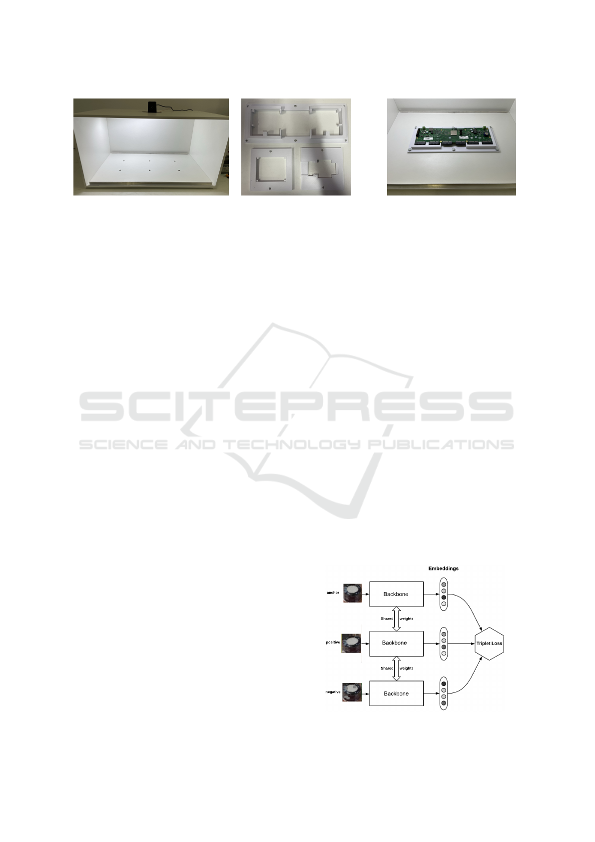
(a) PCB inspection cabinet. (b) Three cradles. (c) Cabinet with a cradle installed.

Figure 2: Elements constituting the hardware developed for this project. (a) Cabinet with 4k camera. (b) Examples of 3D

printed cradles. (c) PCB installed into a cradle.

1. Select an image from a class different from the

anchor.

2. Use a modiﬁed version of the same anchor image,

like the addition of random gray patches.

3. Use a hybrid scheme where both strategies 1 and

2 are combined.

The augmentation routines were planned to allow

the model to discern between correct and incorrect

or defective components, but also to make the model

more robust to naturally occurring small translations

and rotations for non-defective components. At the

end, we were able to generate approximately 4,000

triplets.

2.2 Hardware

A custom cabinet was designed and built to enable

PCB photos to be taken in a controlled environment,

avoiding outside interference and thus ensuring the

correct operation of the model. This kind of cabinet

is designed to be used in real industry environments,

which allows us to test our model in an ambient that

mimics a real scenario.

The cabinet (Figure 2a) is a box built with MDF

(Medium-Density Fiber-board), with an open front.

The box has six holes with nuts at the bottom, al-

lowing cradles for the PCBs to be screwed onto the

bottom. This approach allows the cradle to remain

ﬁxed during PCB veriﬁcation and makes it possible

to change for other cradles associated with different

PCB clients.

The cradle is custom-made and can be printed us-

ing a 3D printer, allowing the user to design an spe-

ciﬁc cradle for each PCB design. This strategy al-

lows us to place different PCBs of the same type in

the same position on the cabinet. We used the GT-

MAX3D CORE GT4 printer and white ABS ﬁlament

to print the cradles used during the experiments (Fig-

ure 2b).

At the top of the cabinet there is an opening where

a Logitech BRIO 4K resolution camera where placed.

An LED strip was installed on the ceiling to provide

a more homogeneous light. It is possible to see in the

Figure 2c the cabinet with a cradle installed during a

PCB inspection.

2.3 Web Application

After model training (cf, Section 2.4), it is inserted

into a web application that can perform the inspection

of the PCBs and manage all the metadata related to it.

The system manages recipes which contains informa-

tion related to the conﬁdence threshold of each com-

ponent. Additionally, there is also the management

of components, which deﬁnes the positive examples

for each component class. This application illustrates

how it is possible to tackle industrial problems by

combining modern NN models with traditional appli-

cation development.

2.4 SNN

Regarding the model, we choose a SNN classiﬁer,

because it is a metric-based model which allows the

addition or removal of classes without being neces-

sary to retrain the model. We performed the training

Figure 3: Our model architecture.

VISAPP 2023 - 18th International Conference on Computer Vision Theory and Applications

892

and validation several times using the grid-search al-

gorithm to ﬁnd the best set of hyperparameters. The

training process was executed by successively insert-

ing positive and negative examples as inputs into the

model.

Since the SNN is a metric-based model, it has the

capacity of comparing two inputs and evaluate if they

are similar or not. So, if we provide two images as

input to the model, it will process both entries and

compare them by using a comparison function that is

deﬁned in its architecture. The SNN training process

is done by using triplet loss, which is deﬁned in the

Eq. (1).

L (I

, I

) = max(∥ f (I

) − f (I

)∥

−

∥ f (I

) − f (I

)∥

+ α, 0)

(1)

Where: f is the network embedding; I

, I

and I

are

the entries (images), and; α is the margin. By opti-

mizing parameters to reduce the triplet margin loss,

the training procedure tries to decrease the distance

between positive and anchor and increase the distance

between negative and anchor. This approach was in-

spired in the FaceNet (Schroff et al., 2015), since they

try to solve a similar problem. The model architecture

can be seen in the Figure 3.

The architecture consists basically of a backbone,

with parameters shared by all the model entries. The

backbone processes the input and summarizes the

most relevant information which are then ﬂattened

into the feature vectors and are compared by the

loss function. We tested four different backbone

topologies, as an attempt of understand which one is

most suitable to extract relevant features from the in-

puts. Those were; InceptionResnet V2; MobileNet

V3 Large; MobileNet V3 Small and ResNet50.

2.5 Evaluation Metrics

The output of the trained SNN was deﬁned in two

categories: nonconformity (N) and conformity (P).

The nonconformity category determines that at least

one of the PCB components is defective or missing.

The conformity category means that all components

are where they were expected to be in the PCB,

determining that such PCB was assembled correctly.

Besides that, the classiﬁcation results were assessed

by analyzing the Precision×Recall curve, computed

by the equations 2 and 3, below.

Prec =

T P

T P + FP

(2)

and

Rec =

T P

T P + FN

, (3)

where, T P denotes True Positive, FP False Positive,

and FN False Negative. The Precision×Recall (PR)

curve was computed using different thresholds of the

similarity score δ between a pair of images. We

also use the Receiver Operating Characteristic Curve

(ROC) and Area Under the Curve (AUC) to evaluate

model performance.

2.6 Experiments

We divided the experiments into two stages aim-

ing at reducing the number of hyperparameters

and, consequently, the number of experiments

necessary to search for the best performance.

In the ﬁrst stage, the selected hyperparameters

were: 1. Enable/Disable batch normalization;

2. Enable/Disable embeddings normalization,

and; 3. Which layers must be trained in the

backbone. Our reason to select these three was be-

cause they were closely related: the backbone used

dictates how many layers we can ﬁne-tune, for exam-

ple. The hyperparameters used in the ﬁrst phase can

be seen in the Table 3.

We began the experiments with two most frequent

categories: Resistor and Capacitor. After that, we per-

formed more experiments where we added the next

class with the highest number of samples to each new

experiment, while using those hyperparameters val-

ues from the best results in the ﬁrst stage.

To enable better experiments, we used the

Lightning (Falcon and The PyTorch Lightning team,

2019) framework to implement and train the model

and timm (Wightman, 2019) to load the pretrained

MobileNet v3 model. The Lightning framework al-

lows us to easily train and test the model, as well as to

Table 3: Hyperparameters used in the ﬁrst phase of the ex-

periments. Others were implemented (e.g., TTA), but not

used.

Hyperparameter Value

Augmentation strategy coarse-dropout-v1

Backbone MobileNet v3 (large, 100)

Batch normalization {True, False}

Batch size 64

Embedding dimension 512

Embeddings normalization {True, False}

Image size 128×128

Learning rate 0.01

Loss function Triplet Margin Loss

Number of epochs 100

Optimizer Adam

Trainable layers {0, 1, 10, 27, 43, 67, 91,

103, 107, 108, 109}

Triplet distance Euclidean

Triplet margin 0.2

Triplet strategy same

Industrial Visual Defect Inspection of Electronic Components with Siamese Neural Network

893

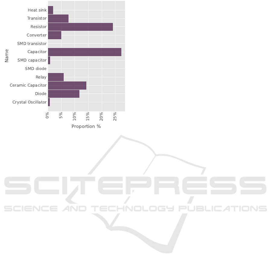
Figure 4: The dataset sample distribution histogram.

use many variations of datasets if needed. The timm

library is a collection of PyTorch modules for com-

puter vision, which allows us to load any pretrained

model and use it in our experiments. For experiment

tracking we used guildai package (Smith, 2018),

which also enable us to perform hyperparameters tun-

ing and compare experiments.

Since our dataset images vary in shapes, we

needed to resize them before passing as input to

the model. We determined the default shape as

128×128×3 because almost 90% of the dataset has

width and height below 128. A batch size of 64

samples (triplets) allows us to introduce class vari-

ety without inserting too much noise. We imple-

mented and used the TripletMarginLoss with default

euclidean distance, but with a customized margin as

hyperparameter (Musgrave et al., 2020). At the end,

we also implemented the Test-Time Augmentation as

an option to the validation stage aiming at decreas-

ing validation metrics variance, because our negative

samples are artiﬁcially created with image processing

augmentation routine.

3 RESULTS AND DISCUSSION

3.1 Database Statistics

Each experiment was tracked and monitored via

guildai and TensorBoard (Abadi et al., 2016),

which allow us to compare the experiment’s metrics

by visualizing the training and validation losses, as

well as image similarity metrics. Figure 5 shows the

training and validation losses of the baseline model,

which was trained using the MobileNet v3 (large,

100) backbone. In addition, we stored the confusion

matrix, distance, and similarity histogram between

pairs in the triplet, PR and ROC curves, and model

weights to evaluate any major changes in the updates.

The database has 18,303 samples (images of elec-

tronic components of PCB) extracted from internet

sources. These images were collected from the Inter-

net using a web crawler developed for this purpose.

The database was divided into 12 classes, as speci-

ﬁed in Table 1. The database distribution among the

classes can be seen in Figure 4. To better observe the

improvement of the model, we determined the valida-

tion set at the beginning of the model development.

3.2 Experiments

Results from the best experiments in phase one (base-

line) are shown in Table 4. We validated the model

based on its accuracy, precision, and recall. Some in-

stabilities are present in the validation, with accuracy

varying from 0.65 to 0.96. We also stored the area

under the Receiver Operating Characteristic (ROC)

curve during validation to inspect the model’s abil-

ity to detect conformities for a given probability of

false positive (see Figure 5a). Similarly, we also plot

a Precision×Recall (PR) curve to analyze their trade-

off, as shown in Figure 5b.

We also evaluated the results using a confusion

matrix, as shown in Figure 5c. The confusion ma-

trix shows us that our model correctly predicted 981

(36.50%) negative pairs and, 1321 (49.14%) positive

pairs. However, there were 23 (0.86%) false nega-

tives and 363 (13.50%) false positives. These results

are detailed in Figure 6, which shows the similarities

between the positive and negative pairs.

In Table 4 we summarize phase 1 by showing only

the best models which achieved an accuracy above

70%, which is a subset of 7 experiments from a total

of 44 that we performed. Except for the experiments

1, 3, and 6, the remaining trials show errors and met-

rics curves similar to the best experiment from phase

Finally, in Table 5 we show the results for phase

2, where we add one more class to each experiment.

We also rerun the experiment which gave us the best

result from phase 1 with purposes of comparison. The

instability showed in the training and validation stages

of the experiments of phase 1 is also present in the

experiments of phase 2. As shown in Figure 1, our

augmentation in the negative sample (middle column)

was intended to mimic defective components, while

the positive sample received a small augmentation.

VISAPP 2023 - 18th International Conference on Computer Vision Theory and Applications

894

Table 4: Metrics for the top models.

experiment amount layer trainable batch norm normalize train/accuracy train/precision train/recall val/accuracy val/precision val/recall

1 67 no no 0.9995 0.9991 1.0 0.9561 0.9268 0.9918

2 91 yes yes 0.9281 0.8810 0.9995 0.8563 0.7858 0.9828

3 91 yes no 0.9894 0.9863 0.9928 0.7511 0.6708 0.9903

4 103 yes yes 0.9967 0.9939 0.9997 0.7395 0.6586 1.0

5 109 yes yes 0.9990 0.9981 1.0 0.7358 0.6563 0.9955

6 108 no no 1.0 1.0 1.0 0.7072 0.6314 1.0

7 108 yes yes 0.9995 0.9993 0.9997 0.7034 0.6289 1.0

What is worse, the results from the best experiment

in phase 1 (experiment 1 in Table 4) could not be re-

produced in a new run (2 in Table 5). These results

seem to indicate that the augmentation may not be

good enough, since the model does not converge as

we expect.

4 CONCLUSION

We presented results of a visual inspection system fo-

cused on electronic components for the purpose of

PCB production quality control. The project was de-

True Positive Rate

False Positive Rate

(a) ROC curve.

Precision

Recall

(b) Precision×Recall (PR).

Figure 5: Baseline results.

veloped in a partnership with a multinational PCB

manufacturing company which possesses a wide va-

riety of international clients.

We developed a complete system — a web app, a

machine learning model, and a hardware plataform —

which enabled the company to inspect defects in un-

seen components. This is a major advantage over cur-

rent rigid inspection process. An SNN architecture,

which is a ﬂexible and scalable solution is adequate to

tackle the problem, was trained using with data gath-

ered from the company and from a web crawler, cus-

tomized for the purpose of collecting images of elec-

tronic components from the internet. The model was

evaluated using a set of experiments showing promis-

ing results.

The overall system is currently deployed in the

company’s manufacturing plant. Its feasibility and

adequacy of the method was demonstrated on a rel-

evant scenario, which can categorize the solution

within a level 6 of Technology Readiness Level

(TRL). Further experiments are being conducted in

a more challenging scenario (production — aimed at

TRL 7) and newer results will be eventually reported.

One of the main obstacles in the development of

the system was the lack of images of non-conform

components. To overcome this problem, we devel-

oped an simple augmentation strategy to simulate de-

fects that could be seen in production by modifying

random regions of the image and adding gray patches.

More work is needed in this vein, that is, how could

we best simulate defects that would generalize well

for all types of components? Each component has its

own rules for what can be categorized as an defect.

For example, a capacitor can’t be rotated by 180 de-

grees, but a resistor can.

Another fruitful approach is to use other distances

and losses for the SNN model. The current model

uses a triplet loss function with a default euclidean

distance, which is a common strategy in the metric

learning literature. Also, a common loss in the face

recognition literature, the ArcFace loss (Deng et al.,

2019), could be used.

At the end, we think that by curating better data,

developing a new augmentation strategies, and taking

advantage of the training scripts we implemented, our

work can be used in the industry to improve the qual-

ity control process of PCB production.

Industrial Visual Defect Inspection of Electronic Components with Siamese Neural Network

895

Figure 6: Histograms of cosine similarities for negative (left) and positive (right) pairs.

Table 5: Metrics for the top models in phase 2.

experiment classes train/accuracy train/precision train/recall val/accuracy val/precision val/recall

1 Resistor, Capacitor, Capacitor Cer

amico 0.9855 0.9727 1.0 0.7199 0.6423 1.0

2 Resistor, Capacitor 0.9968 0.9942 0.9996 0.6860 0.6170 0.9903

3 Resistor, Capacitor, Capacitor Cer

amico, Diodo 0.9991 0.9989 0.9993 0.5554 0.5295 1.0

ACKNOWLEDGEMENTS

This work was partially funded by SOFTEX

REFERENCES

Abadi, M., Agarwal, A., Barham, P., Brevdo, E., Chen, Z.,

Citro, C., Corrado, G. S., Davis, A., Dean, J., Devin,

M., et al. (2016). Tensorﬂow: Large-scale machine

learning on heterogeneous distributed systems. arXiv

preprint arXiv:1603.04467.

BROMLEY, J., BENTZ, J. W., BOTTOU, L., GUYON,

I., LECUN, Y., MOORE, C., S

ACKINGER, E., and

SHAH, R. (1993). Signature veriﬁcation using a

“siamese” time delay neural network. International

Journal of Pattern Recognition and Artiﬁcial Intelli-

gence, 07:669–688.

Deng, J., Guo, J., Xue, N., and Zafeiriou, S. (2019). Ar-

cface: Additive angular margin loss for deep face

recognition. In Proceedings of the IEEE/CVF con-

ference on computer vision and pattern recognition,

pages 4690–4699.

Falcon, W. and The PyTorch Lightning team (2019). Py-

Torch Lightning.

Harris, M. (2022). These 5 charts help demystify the global

chip shortage.

alber, F., K

ukl

u, O., Lehment, N., and Rigoll, G.

(2021). U-net based zero-hour defect inspection of

electronic components and semiconductors. pages

593–601. SCITEPRESS - Science and Technology

Publications.

Luan, C., Jing, Z., and Zuo, J. (2021). A defect-sensitive

loss function based on siamese network to defect de-

tection with imbalanced samples. Journal of Physics:

Conference Series, 1802(4):042085.

https://softex.br/

Musgrave, K., Belongie, S., and Lim, S.-N. (2020). Pytorch

metric learning.

Nagy, A. and Cz

uni, L. (2021). Detecting object de-

fects with fusioning convolutional siamese neural net-

works. pages 157–163. SCITEPRESS - Science and

Technology Publications.

Pramerdorfer, C. and Kampel, M. (2015). A dataset for

computer-vision-based pcb analysis. In 2015 14th

IAPR International Conference on Machine Vision

Applications (MVA), pages 378–381. IEEE.

Reza, M. A., Chen, Z., and Crandall, D. J. (2020). Deep

neural network–based detection and veriﬁcation of

microelectronic images. Journal of Hardware and

Systems Security, 4:44–54.

Saeedi, J. and Giusti, A. (2022). Anomaly detection for

industrial inspection using convolutional autoencoder

and deep feature-based one-class classiﬁcation. pages

85–96. SCITEPRESS - Science and Technology Pub-

lications.

Schroff, F., Kalenichenko, D., and Philbin, J. (2015).

Facenet: A uniﬁed embedding for face recognition

and clustering. In Proceedings of the IEEE conference

on computer vision and pattern recognition, pages

815–823.

Smith, G. (2018). Guild ai - experiment tracking, ml devel-

oper tools. https://github.com/guildai/guildai.

Tang, S., He, F., Huang, X., and Yang, J. (2019). Online

pcb defect detector on a new pcb defect dataset.

Wightman, R. (2019). Pytorch image models. https:

//github.com/rwightman/pytorch-image-models.

VISAPP 2023 - 18th International Conference on Computer Vision Theory and Applications

896