Exploring False Demand Attacks in Power Grids with High PV

Penetration

Ashish Neupane

and Weiqing Sun

The University of Toledo, 2801 Bancroft St., Toledo, OH, U.S.A.

Keywords: False Data Injection Attacks, Kalman Filter-based Detector, High PV Penetration, False Demand Attacks,

Dynamic Threshold Detectors.

Abstract: The push for renewable energy has certainly driven the world towards sustainability. However, the

incorporation of clean energy into the electric power grid does not come without challenges. When

synchronous generators are replaced by inverter based Photovoltaic (PV) generators, the voltage profile of

the grid gets considerably degraded. The effect in voltage profile, added with the unpredictable generation

capacity, and lack of good reactive power control eases opportunities for sneaky False Data Injection (FDI)

attacks that could go undetected. The challenge is to differentiate these two phenomena. In this paper, an

attack is explored in a grid environment with a high PV penetration, and challenges associated with designing

a detector that accounts for inefficiencies that comes with it is discussed. The detector is a popular Kalman

Filter based anomaly detection engine that tracks deviation from the predicted behaviour of the system. Chi-

squared fitness test is used to check if the current states are within the normal bounds of operation. We identify

the vulnerability in using static and dynamic threshold detectors which are directly affected by day-ahead

demand prediction algorithms that have not been fully evolved yet. Finally, we use some of the widely used

machine learning based anomaly detection algorithms to overcome the drawbacks of model-based algorithms.

1 INTRODUCTION

The electric power grid has seen a lot of changes in

recent years. Traditionally, power system comprised

of synchronous generators with high power

generation capability and a predictable voltage profile

that fluctuated slightly throughout the day. These

synchronous generators almost exclusively provided

the bulk system voltage regulation. However, that is

quickly changing, and with the synchronous fossil

fuel and nuclear-powered generators being retired

slowly but steadily, it has led to the need for

renewable generation to contribute more significantly

to the power system voltage and reactive regulation

(McDowell & Walling, 2016).

The synchronous generators reliably produce

reactive power by controlling the excitation current

through the rotors. Although there is a limit to the

magnitude of field current that can be supplied to

rotor windings of a generator to produce reactive

power, its production has little effect on the terminal

https://orcid.org/0000-0001-8481-7306

https://orcid.org/0000-0002-6973-0509

voltage of the generator. That helps the synchronous

generators achieve a good voltage profile.

On the other hand, due to the limited converter

current capacity of PV, its reactive power capacity is

usually smaller compared with that of a synchronous

generator, especially when PV’s real power output is

close to the rated value. Inverters used for solar PV

and wind plants can provide reactive capability at

partial output, but any inverter-based reactive

capability operating at full power implies that we

need a larger converter to handle full active and

reactive current (Till et al., 2020). This means either

the PV generators would have to operate significantly

lower than their maximum rated output, or make a

trade-off in the voltage.

The grid is changing substantially with the

introduction of Distributed Energy Resources (DER)

and wide adoption of renewables. With these ongoing

changes in the grid, the traditional definition of grid

stability is not always applicable. Most of today’s

infrastructure is internet accessible, and false data

124

Neupane, A. and Sun, W.

Exploring False Demand Attacks in Power Grids with High PV Penetration.

DOI: 10.5220/0011695800003405

In Proceedings of the 9th International Conference on Information Systems Security and Privacy (ICISSP 2023), pages 124-134

ISBN: 978-989-758-624-8; ISSN: 2184-4356

 2023 by SCITEPRESS – Science and Technology Publications, Lda. Under CC license (CC BY-NC-ND 4.0)

injection attacks could give an indication that the

voltage levels on buses with PV generators are very

low, when the generator could be operating normally.

Normally, this would not be a problem, because false

data injection attacks are easily detectable in power

systems with low PV penetration, because these

systems have predictable voltage and current levels.

Since the injections would have voltage/current levels

that vary significantly from the voltage levels at

which synchronous generators operate, a Chi-squared

detector would easily pick up these anomalies. The

same detector would also detect the injection attacks

at systems with high PV penetration, however the

system parameters during normal operation at high

PV penetration when PV generators are close to

maximum power generation limits, and during attacks

at low PV penetration would be indistinguishable to

the detector.

This paper aims at showing an attack scenario that

takes advantage of poor voltage profile during peak

loads at a grid with high PV penetration. We compare

how the traditionally used model-based algorithms

perform against the machine learning based

algorithms in such a condition. For model-based

algorithm, we use Kalman Filter based detector,

which is widely researched in state estimation as well

as detection of attacks. However, unlike other

research, our model is based on day-ahead demand

predictions, which defines the normal operation of the

system and ultimately thresholds for the states at any

given time of the day. The states are highly dependent

on the demand, especially in grids with high PV

penetration, and our model takes that into account to

get a better prediction. However, the crucial part of

our work is showing how model-based algorithms

perform poorly in high PV scenarios with high false

positives.

2 RELATED WORKS

Detection methods for False Data Injection Attacks

have been researched for a few decades. These

algorithms are broadly categorized as model-based

detection algorithms and data-driven detection

algorithms (Musleh, 2020). Duan et al. (2018), Chung

et al. (2017), Inayat et al. (2022), and Jiang et al.

(2017) extensively used Weighted Least Squares

algorithm. These first detectors were static and

iterative in nature, which did not use the last state to

update the new state. That made them slow and

processor intensive. Kurt et al. (2018) and Wang et al.

(2019) used Kalman filters and some of its variations.

Karimipour & Dinavahi (2017, 2018) specifically

used Extended Kalman Filters and were able to

address non-linearity in the system and yielded more

precise estimate. Unlike WLS, these detectors are

dynamic in nature and use the last state to update the

current state.

Some detection algorithms are however

estimation-free. Cooperative Vulnerability Factor

(CVF) employs secondary output of voltage

controllers that converges to zero if the system is

under the FDI attack (FDIA) (Sahoo et al., 2019).

This technique was used in microgrids environment.

Another technique called Matrix Separation (MS)

exploits the sparse nature of FDIA by separating

nominal states of power grid and anomaly matrices

(Li et al., 2019; Liu et al., 2014). Ameli et al. (2019)

and Ashok et al. (2016) presented some similar

techniques. Data-driven detection algorithms are

popular class of algorithms broadly classified as

Machine Learning, Data Mining and other

miscellaneous algorithms. Supervised learning

technique use datasets that have labelled data to

separate attacks from the normal flow. They have

high accuracy but cannot detect new variation of

attacks. Unsupervised learning does not need labelled

data but is extremely difficult to model. Support

Vector Machine (SVM), which is a type of supervised

learning is the most utilized in FDIA. Binna et al.

(2018), Foroutan & Salmasi et al. (2017) and Wang

et al. (2019) have presented works in this area. In the

unsupervised category, K-means clustering is very

popular. The works of Zanetti et al. (2019) and Viegas

& Vieira (2017) are some of the notable ones.

A wide variety of Kalman Filter has been used in

the detection of False Data Injection Attacks. One of

the challenges faced in the research is modelling non-

linear relationship of power and voltages in the grid.

Farsadi et al. (2017) presented dynamic state

estimation that does not require calculation of

Jacobian matrix, which decreases the processing

time. Similarly, Qi et.al (2018) introduced cubature

Kalman Filter (CKF) that has a non-linear observer.

These were then tested on a 68-bus system under

various uncertainties in a realistic scenario. The

authors showed that the model was comparatively

more robust to uncertainties in the systems including

cyber-attacks.

A risk mitigation strategy was presented by Taha

et al. (2018) that addresses dynamics in the system for

higher order depictions by utilizing a dynamic state

estimator. Minot et al. (2019) proposed a unique

approach to dynamic state estimation. The algorithm

employs a fully distributed approach where the

estimation has an innovation design element for

attack detection which reduces the overhead in

Exploring False Demand Attacks in Power Grids with High PV Penetration

125

communication. Zhang et al. (2014) designed an

Adaptive Kalman Filter with Inflatable Noise

Variances (AKF with InNoVa) algorithm that uses a

2-stage system that estimates static states like voltage

magnitudes as well as dynamic states like generator

rotor angles. The first stage of the system filters out

the impact of incorrect system modelling and bad

PMU measurements using AKF with InNoVa. The

result in the first stage is served as a measurement to

the second stage which has an Extended Kalman

Filter (EKF). Manandhar et al. (2014) used Chi-

squared detector to detect anomalies in the system.

The residuals from Kalman filter were fed to a

Euclidean detector which has the parameters for

normal level of the system and detects if there is any

deviation from the normal operation.

However, to our knowledge, none of the algorithms

have been tested in a high PV penetration environment

where, at peak demands, the grid shows behavior

which mimics an attack. The grid supposedly needs to

know the context to a wide number of variables to

predict accurately in such scenario. We test this

hypothesis in this paper and compare model-based

approach with data-driven algorithms.

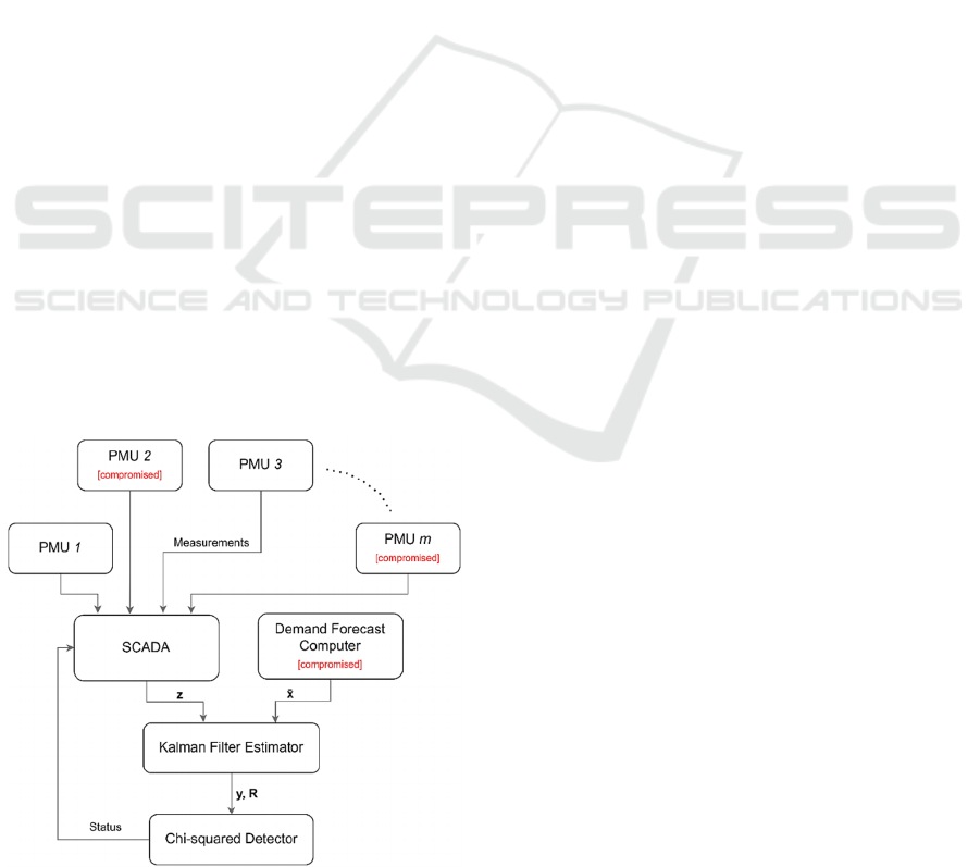
3 SYSTEM MODEL

The system consists of a Supervisory Control and

Data Acquisition (SCADA) system, which gets the

measurements from the Phasor Measurement Units

(PMU) capable of measuring line currents and bus

voltages as well as detection results from a Chi-

squared detector. The system model is shown using

the block diagram in Fig. 1.

Figure 1: Block diagram of the system model.

The measurements from all sections of the grid are

collected and that data is fed to the state estimator

engine, which filters out the measurement and

process errors, and generates the best estimate of the

system. The Chi-squared detector is aware of the co-

variances between different states of the system and

gets the most recent data from the estimator. The

detector then generates the result and sends it back to

the SCADA.

3.1 Kalman Filter Anomaly Detector

The Kalman Filter has been extensively used in

various applications in mathematics, engineering, and

economics. The filter is robust and provides good

estimation of systems. At its core, Kalman filter

balances the prediction of states and measurements of

the states. Based on which of the two has higher

beliefs, process or measurements, the filter calculates

its estimation. It assumes that the measurement error

variance and process covariance is already known.

The prediction equation is given below.



= Fx + Bu (1)



= FPF

+ Q (2)

where,

x and P are the state mean and covariance

F is the state transition function

Q is the process co-variance

B and u are the control inputs which is 0 here

The first equation calculates the current state

based on the last state and the state transition matrix.

The states in the equation are vectors of real and

imaginary voltages given by equation (3).



Re(z)

Im(z)

= 

Re(H)

Im(H)

-Im(H)

Re(H)



Re(x)

Im(x)



Re(v)

Im(v)



(3)

Unlike most of the research, where state transition

matrix is taken as identity matrix because it is

assumed that the next state is the mean of the stable

state and some process error, our research uses pre-

computed factors obtained from the demand forecast

computer. The state transition matrix is derived for

each time step using pre-obtained data from the

demand forecast computer. This data is then used to

simulate the load flow for the grid and get a prediction

of various states for each time step. It should be noted

that estimation is a two-part process: predict and

update.

The prediction step always lessens the belief that

the estimator has towards the system. In other words,

ICISSP 2023 - 9th International Conference on Information Systems Security and Privacy

126

instead of having high probability in a small range of

states, the estimates get dispersed to a slightly wider

range of values with lesser probabilities. That is

corrected by the update state. The measurement

equation is shown using equation 4 below.

y = z - Hx (4)

K = PH

HPH

+ R

-1

(5)

x = x + Ky (6)

P =



I - KH



P (7)

where,

y is the residual

H is the measurement function/matrix

z and R are the measurement mean and noise

covariance

P and K are the state covariance and Kalman gain

The residual y is the difference between measured

values and predicted measurements which have been

derived from the predicted states using H. The

variables K and P converges to some stable values.

The measurement matrix converts the states from the

state space to its corresponding measurements in the

measurements space. The calculation of H matrix has

been explained by Zhang et al. (2010). The

conversion of states to the measurement space

however also changes the covariance. Hence, it needs

to be recalculated in each iteration which is given by

the relation in equation (7). It should also be noted

that although the Kalman gain remains fairly stable

after getting converged, the value should also be

calculated in each state for a more accurate prediction

and to avoid propagation of error.

3.2 Demand Forecast

Although these research works have different

approaches and techniques, most of them have a

similarity in how they assume the states change with

time. Most of the research assumes the states remain

fairly stable, and only change slightly by introducing

a Gaussian noise. While that may be true for very

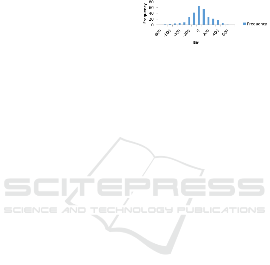
small amount of time, real and reactive power

demand is very dynamic in a grid environment and

there are always errors in demand as shown in Fig. 2.

This fact means that failure to include that in the

system model makes it extremely difficult to model

state changes into the system, and consequently

mistake demand changes for an FDIA.

Our research takes a different approach. At the

core of the system model is a day-ahead demand data

Figure 2: Histogram of day-ahead demand errors.

that drives the state transition function F, and

especially state co-variance Q in the Kalman filter

equation. Predicting demand ahead of time is a highly

complex procedure. Many factors will need to be

considered when generating a load forecast. Some of

these are simple like climate and weather, historical

usage patterns, day of the week, social events,

residential or industrial load, and so on, while others

are complicated like Behind the Meter (BTM). The

Independent System Operators (ISOs) have been

working relentlessly to improve the forecasting

methodologies over the years. In recent days, they

have reached a point where day ahead forecasts were

within 1% of actual peak demand in most of the days

(Reliable Energy Analytics, 2021). The main

challenge currently is accounting for BTM PV supply

resources.

In order to use Kalman filter for state prediction,

the error in predictions should be normally

distributed. There has been a large number of research

as well as implementations for day-ahead power

demand and net-demand predictions. A report by

Reliable Energy Analytics (2021) shows some of the

techniques used by a few ISOs. We did a Shapiro-

Wilk test on the day-ahead predictions used by

California Independent System Operator (CAISO)

using the data published on their website. The

prediction error passed the test, and the corresponding

histogram is shown in Fig. 2. However, our research

uses voltages as states, and because the relation

between voltage and power is non-linear, a normal

distribution would be skewed if such a conversion is

used. Some variations of Kalman filter like Extended

Kalman Filter (EKF) can be used to work with non-

linear systems, but we chose a different route. An

independent voltage prediction algorithm like the one

used by Mokhtar et al. (2021) would predictably have

errors which are normally distributed. We move

forward with that assumption and artificially inject

Gaussian normal process error.

3.3 Chi-squared Detector

The Kalman filter is used in conjunction with a Chi-

squared detector in this research. The Chi-squared

Exploring False Demand Attacks in Power Grids with High PV Penetration

127

detector is widely used for goodness of fit tests. That

makes it practical for use in detecting false data

injections where the normal states of the system can

be plugged in, and with the knowledge of co-variance

in the states, the Chi-squared values can be obtained.

Mo & Simopoli (2010) showed the following can be

computed.





= y

-1

Ry (8)

The measurement covariance matrix R is crucial

in the above equation. If the residual deviates from

expected values, the Chi-squared value goes higher,

indicating an inconsistency between the expected and

real value. The two suspected causes of this

inconsistency are false data injection attacks, and a

switch from synchronous generators to PV

generators, which has a poor voltage profile. The

challenge, and the focus of research is to differentiate

the two.

4 IMPLEMENTATION AND

EVALUATION

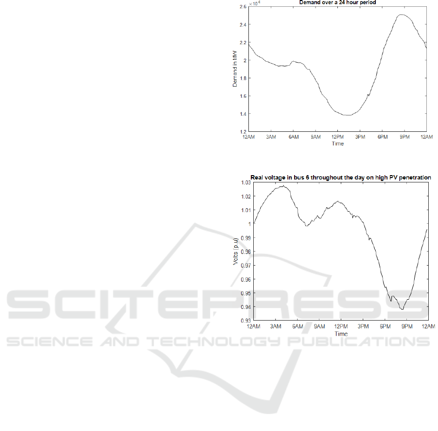
The research is simulated on an IEEE 14 bus with the

standard load profile. A 24-hour demand curve is

extracted from CAISO’s website as shown in Fig. 3

that drives the real and reactive power demands on

each bus. The load flow is solved for each demand,

and the corresponding states are obtained.

4.1 Simulation Setup

In our setup, an IEEE 14 bus is simulated using Power

World Simulator. The simulator runs 24-hour load

demands and calculates the corresponding states and

measurements. The load demand is obtained from

CAISO every 5 minutes totaling 289 demand points.

These data points are interpolated to obtain 5,000 data

points which is imported into MATLAB where

Kalman filter predicts and estimates the real and

imaginary voltages on each bus. The per-unit real

voltage on bus 6 over 24-hour is shown in Fig. 4.

The load flow is solved using the MATPOWER

package. The Newton’s method is used to solve non-

linear load flow equations. The Kalman filter

estimator gets measurement data from the load flow

solution and makes estimates using the day-ahead

predictions and measurements. The reactive power

generation in any power system is restricted by the

reactive capability curve. The general idea behind

reactive capability curve is that, for any given amount

of active power generation, there is a limit on the

Figure 3: Power demand over a 24-hour period.

Figure 4: Voltage levels over a 24-hour period in bus 6.

amount of reactive power that can be generated. The

limit is determined by the capability curve. Fig. 5

shows the operating area of the PV inverters which

are highly restricted by the power factor requirements

and internal limits. The reactive power generation is

limited in PV inverters, and although they can have

D-shaped curve, this is not an industrial standard

(Mcdowell & Walling, 2016).

There is a special STATCOM mode which allows

the PV inverters to generate reactive power without

producing any active power and use that for voltage

regulation. However, this mode is not always

available due to restrictions. The reactive capability

curve of the operating range was inserted into the

Power World Simulator using a piecewise linear

model. The PV control model, while being a crucial

part of the system, has limited scope in our research

and its intricacies are almost independent on how the

attacks are carried out. Hence, it is excluded.

The simulation setup for machine learning based

detector is highly rigorous because unlike model-

based algorithms where the states would be calculated

ICISSP 2023 - 9th International Conference on Information Systems Security and Privacy

128

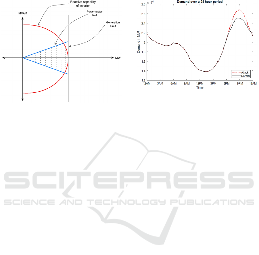
Figure 5: Reactive capability curve of PV generator.

using an equation, machine learning algorithms rely

on pre-simulation of all the load flow condition that

the model may encounter in real life.

4.2 Attack Model

The false data injection attack is carried out by

changing the measurements on a PMU unit. This

paper assumes that the attacker has access to a limited

number of PMUs in the grid and is able to manipulate

bus voltages and line current measurements on that

PMU. As proposed by Abur & Expósito (2004), any

unsophisticated attack can be easily detected using

plausibility tests. Some red flags include voltage

magnitudes that are negative or considerably higher

or lower than the operating range of the bus, failed

KVL and KCL tests and power equations.

Any sophisticated attack would easily pass those

tests. Hence, we are exposing a difficult-to-detect

attack, which makes the detection extremely hard.

The attack impersonates a drop in voltage due to poor

reactive performance that results in a less ideal

voltage profile of PV generators. This attack is

specifically targeted at a system that has higher PV

penetration. Till et al. (2020) showed how the

increase in penetration of PV generators results in a

poor voltage performance.

In the attack, as shown in Fig. 6, the attacker can

get the bad voltage profile measurements and inject it

during the time when the grid is performing normally.

The detector will have difficulty in differentiating

if the anomaly is caused by an attack or the high PV

penetration. The challenge with this kind of attacks is

that there should be no visible transition between a

normal operation and the attack. A sudden drop in

voltage, or a sudden loss in a portion of the grid is a

Figure 6: False demand injected by the attacker.

major red flag that will draw immediate attention. We

assume that the attacker can access demand forecasts

on a generator bus which is being attacked. The

access can be obtained by compromising a computer

which stores demand forecasting information. The

attacker can even go a step further and run their own

demand forecast algorithm using the historical data

and the freely available machine learning tool.

The PV generators’ voltage drops quickly when

approaching active and especially reactive power

generation limit (Till et al., 2020). The data in the

demand forecast could be compromised and give a

false impression that the demand is increasing. This

helps justify the voltage drop across busses. The

reason that helps make the attack successful is that it

blends in with the poor voltage control of PV

generators. The timing of the attack during peak

summer hours could even make it go unnoticeable.

4.3 Calculation of Kalman Filter

Parameters

The states in Kalman filter are the parameters whose

estimations are done by balancing the value between

its measured and predicted versions. The states in this

work are all the real and imaginary voltages in a 14-

bus setup. The following expression shows the states

of the setup.

x =











. .Im





. . Im(V14)



(9)

There are n states in the system. Hence, the size

of x is n×1. When the simulation starts, the states

have to be initially set to a certain stating condition.

Usually, the rule of thumb is to start the states with a

flat start condition. The states are initialized by setting

all the real voltages to 1 and all the imaginary voltages

to 0. However, the states of the grid are tentatively

known and hence, the grid configuration is pre-

Exploring False Demand Attacks in Power Grids with High PV Penetration

129

simulated to get the stable values of the states, which

results in faster convergence.

The state transition matrix defines the transition

of states from current state to next state (Labbe,

2020). The grid is a very dynamic infrastructure, and

hence it is extremely difficult to accurately predict the

next state of the system based on the current state.

However, in this case, because the states are voltages,

the Automatic Voltage Regulation (AVR) system

always tries to stabilize the voltage between ±5% of

the nominal voltage of 1 P.U, and hence, it is easier

to compute the state transition matrix.

This research work uses a different approach in

calculating F based on the real-world scenario.

Unlike other research where states are modelled to

vary randomly between certain ranges, the work takes

into account that the grid has a dynamic active and

reactive power demand that varies throughout the

day, and it affects the states of the system based on

whether majority of its power comes from

synchronous generators or PV generators. The day-

ahead demands throughout the day is download from

California Independent System Operator (CAISO),

simulated on an IEEE 14 bus configuration and the

matrix F is calculated for each time step. However,

the research work would be of no use if F was made

to be 100% accurate. Instead of using hour-ahead

demands for F, day-ahead demands are used. And

because day-ahead demands are slightly inaccurate

than hour-ahead demands, there is a need for

accurately predicting the next state by using

measurements. For instance, the next state from the

current state is calculated as follows:

x = 



x = 





State transition matrix is a n×n matrix. Here, the

second equation predicts the next state using F. The

state x

changes by a factor of A and x

changes by a

factor of B. It is assumed that the states transition only

depend the state itself and not on other states, the off-

diagonal elements of F are 0. However, in a grid, the

states do depend on the values of other states which

has to be taken into account. That is done by

incorporating state co-variance P and process

covariance Q.

As discussed earlier, the state transition matrix

takes time-dependent state transitions into account

which is part of the process. Kalman filter also has B

and u that considers any known external forces or

variables, which is ignored in this work. However, the

possibility of any unknown variables changing the

predictions is huge. The filter should be designed in a

way that expects some unaccounted variables and

models uncertainty using it as a variable in the

equation. The process covariance Q helps the filter

account for those uncertainties.

The modelling of Q matrix is very crucial and one

of the most difficult tasks of a Kalman filter and it is

important to model Q accurately. If Q is too low, the

filter will have more confidence in the prediction

model and ignore noises in the system. If it is too

high, the filter becomes inaccurate because its

prediction will be largely influenced by the noise

(Labbe, 2020). While there are various approaches to

calculating Q, the appropriate Q matrix was obtained

in this work by simulating the IEEE bus under various

load conditions and evaluating the errors obtained in

the simulation. When following this method, the

simulation should be iterated numerous times to

account for various load conditions and uncertainties

in the grid.

The measurement covariance R represents the

predicted observation errors. This is sometimes

referred as sensor noise and can be estimated easily

by comparing the expected results with the sensor

measurements (Labbe, 2020).

The state covariance matrix P shows the relation

between all the system states. Mathematically, it is a

measure of joint probability of two random variables.

The covariance is defined as:

cov



X, Y



= E[



X-E







Y-E







] (10)

where, E[X] is the expected value of random

variable X.

A positive value of covariance between two

variables, or state in this case shows a direct relation

between those state and a negative value indicates

inverse relationship. The matrix P is initialized in the

Figure 7: State covariance convergence.

similar way to the states. It doesn’t have a strict

requirement like Q because P is optimized in each

time step of Kalman filter equations, and ultimately

ICISSP 2023 - 9th International Conference on Information Systems Security and Privacy

130

converges to a stable value (Labbe, 2020) as shown

in Fig. 7.

The state covariance matrix P is a symmetric

matrix of size n×n where the element P

shows the

relationship between states i and j. The Kalman filter

equations have n states and m measurements. The

measurements done on the system can be different

from the states. Therefore, in order to get a residual

value between the predicted states and measurement,

all the states have to be converted to the measurement

space to make mathematics compatible to the same

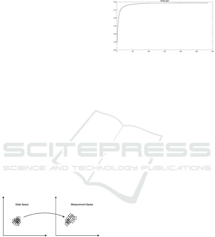
operands. Fig. 8 illustrates this concept where the data

points on the state space are converted to datapoints

in measurement space using the measurement

function H.

In order to convert states x to its measurement

counterparts z, the m×n matrix H should be chosen

such that the resulting operation Hx gets converted to

measurements with elements V1, V5 and V8. Hence,

it is necessary to first come up with a relationship

between different voltages.

z –

y = 

 H 



The Kalman gain decides whether the estimation

should lean towards predicted values or measured

values based on which value the filter has higher

confidence in (Labbe, 2020). Kalman gain also

converges to a stable value as shown in Fig. 9. In

matrix form, the Kalman gain is a n×m matrix which

sums each product between Kalman gains and

measurements for a particular state.

Figure 8: Conversion from state to measurement space.

4.4 Detection Using Model-based

Algorithms

The attack model was simulated on Power World

Simulator and MATLAB. During the period of the

attack between 6 PM and 11 PM, a false demand is

injected by the attacker where the demands are made

to go higher than expected. The detector has a static

Figure 9: Kalman gain convergence.

threshold level that determines the normal operation.

Any voltage levels above or below the normal

operating ranges will be picked up by the detector and

the Chi-squared value goes higher as the difference

between expected values and measured values goes

high. As Fig. 10 shows, the Chi-squared values kept

rising and ultimately exceeded the threshold during

the attack.

This was an expected behavior. However, running

a separate simulation with high PV penetration during

the interval of the attack, the graph was similar and

indistinguishable. This gives the realization that

under high PV penetration grid environment, a Chi-

squared detector alone cannot be used as a detector

because it will give many false positives. As the

system switches from solar to synchronous depending

on the generation capabilities, more false detection

alarms will be generated.

The results show that the detector is not able to

differentiate an attack from the poor voltage profile

of the PV generator. The top graph is simulated with

an attack, and the bottom graph is simulated with the

generator switched from synchronous to PV. Hence,

a traditional Chi-squared based detectors will raise a

large number of false positives if deployed in grids

with high PV penetration. A simple solution would be

modifying the Kalman filter model to expect voltage

degradation due to the switch to PV.

However, the problem with this approach is that

the attacker now has more flexibility for attacks even

when PV penetration is low and can easily carry out

attacks without the detector even noticing it. Another

solution could be changing the Kalman filter model

dynamically depending on the % of PV penetration in

the system. While this solution can accurately detect

attacks, the switch to PV in most of the plants is

unpredictable, and if the SCADA is compromised, the

detector is useless.

A slightly different approach was taken by Wang

et al. (2022). Dynamic threshold is used based on the

false alarm rate allowed at the current moment instead

of the static threshold. This allows adjusting the

Exploring False Demand Attacks in Power Grids with High PV Penetration

131

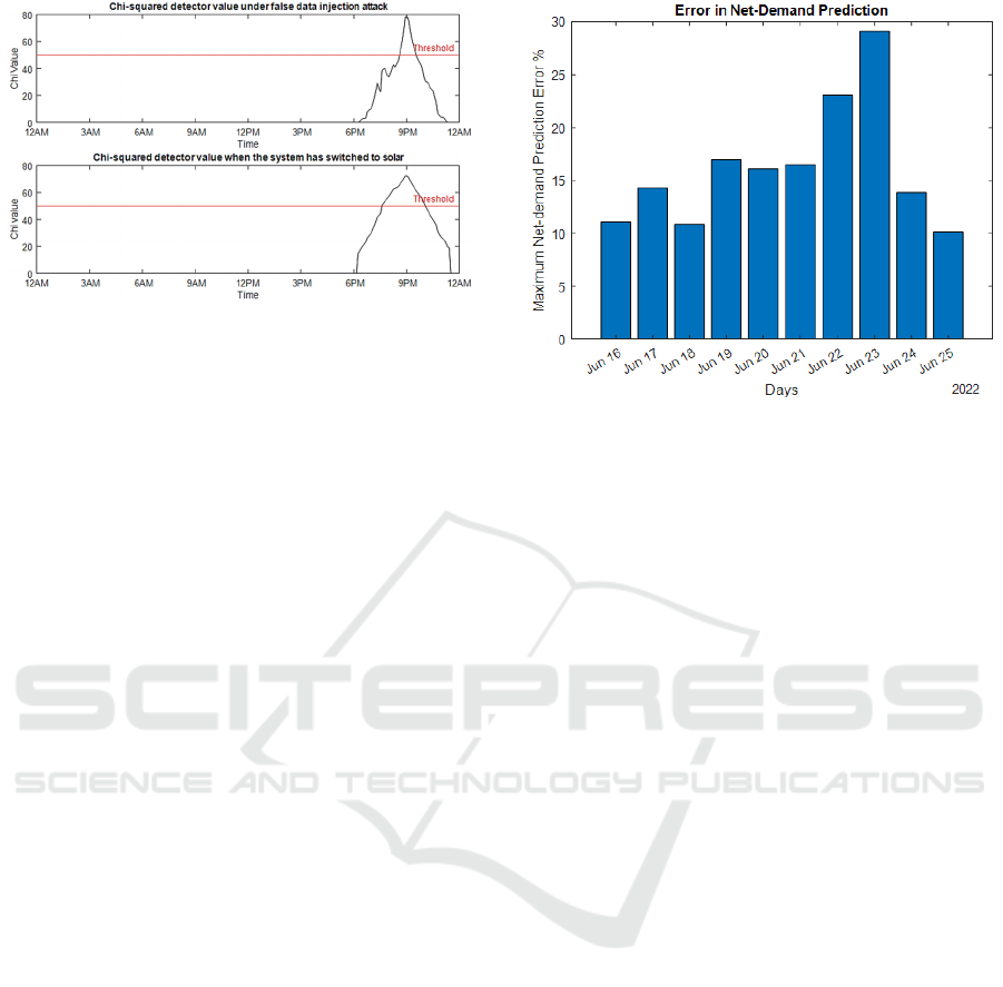
Figure 10: Chi-squared values during attacks vs high PV

penetration.

false alarm rate during periods where solar

penetration is high. However, solar generations and

net-demand is difficult to predict accurately. Wang et

al. (2022) mentioned that the yin-yang effect of

Behind the Meter (BTM) PV adversely affects the

net-demand prediction. Whatever BTM PV supply

does not get produced (i.e., due to weather), will

likely result in an increase in demand/load

approximately equal to the missing BTM supply.

Hence, the load forecasting algorithm continuously

misses its day-ahead net demand forecast. The

algorithm is only as good as the data provided to it,

and with the increasing number of customers using

BTM solar plants, the algorithm needs access to data

from these plants in real time to predict accurately.

This is currently not feasible because there are too

many variables to keep track of, and there is

inconsistency in the available customer data.

Fig. 11 shows maximum errors in net-demand

prediction over 10 days between June 16 and 25, 2022

in the data published by CAISO. On 23

of June, the

maximum error was close to 30%. It only backs our

concern that dynamic threshold-based detectors

cannot be relied on to make estimations, which makes

them equally, if not more vulnerable than static

threshold-based detectors. This is not the only issue

that makes demand predictions unreliable. Various

kinds of faults can change the topology of the network

and alter the power demand at a particular generator.

The faults are random in nature and is almost

impossible to predict accurately.

4.5 Detection Using Machine Learning

Algorithms

We have explored four widely used anomaly

detection algorithms based on Machine Learning to

learn the behavior of the grid under varying load

condition and % PV penetration. The training dataset

Figure 11: Errors in day-ahead prediction over a 10-day

period.

includes 12 load demands from all months of the year

derived from California Independent System

Operator. Each 24-hour demand is then divided into

5000 loads, and each load on the grid changes

proportional to that load demand. The crucial part of

this simulation is that the same simulation is done

multiple times from 0%-100% PV penetration. The

load flow data used for simulation are per unit

voltages and MVAR generation and demand. Hence,

the grid not only knows how to correlate the grid

parameters, but any attempt to inject portions of

parameters like voltages and power demands is

detected by the anomaly detection model. The

training model is depicted using Fig. 12. Table 1

compares the FDIA detection capabilities of machine

learning and Kalman filter algorithms under 0% PV

penetration, while Table 2 compares the algorithms

when there is FDI attack, and the grid is operating

under 80% PV penetration. A crucial part of our work

is exploring the behavior of machine learning

algorithms when the grid is switched to solar.

Specifically, we are interested in observing if the

algorithm can differentiate higher PV penetration and

false data injection attacks, which the Kalman Filter

based algorithm failed to do.

As seen in Table 1 and 2, One-class Support

Vector Machine (OCSVM) algorithm has the best

accuracy among all the machine learning algorithms,

but also gives higher amounts of false positives. As

the Table 2 shows, the machine learning algorithms

have substantially lower false positive rate than

Kalman Filter which indicates that the poor voltage

profile during high PV penetration condition is ruled

not as attack but to higher solar penetration.

ICISSP 2023 - 9th International Conference on Information Systems Security and Privacy

132

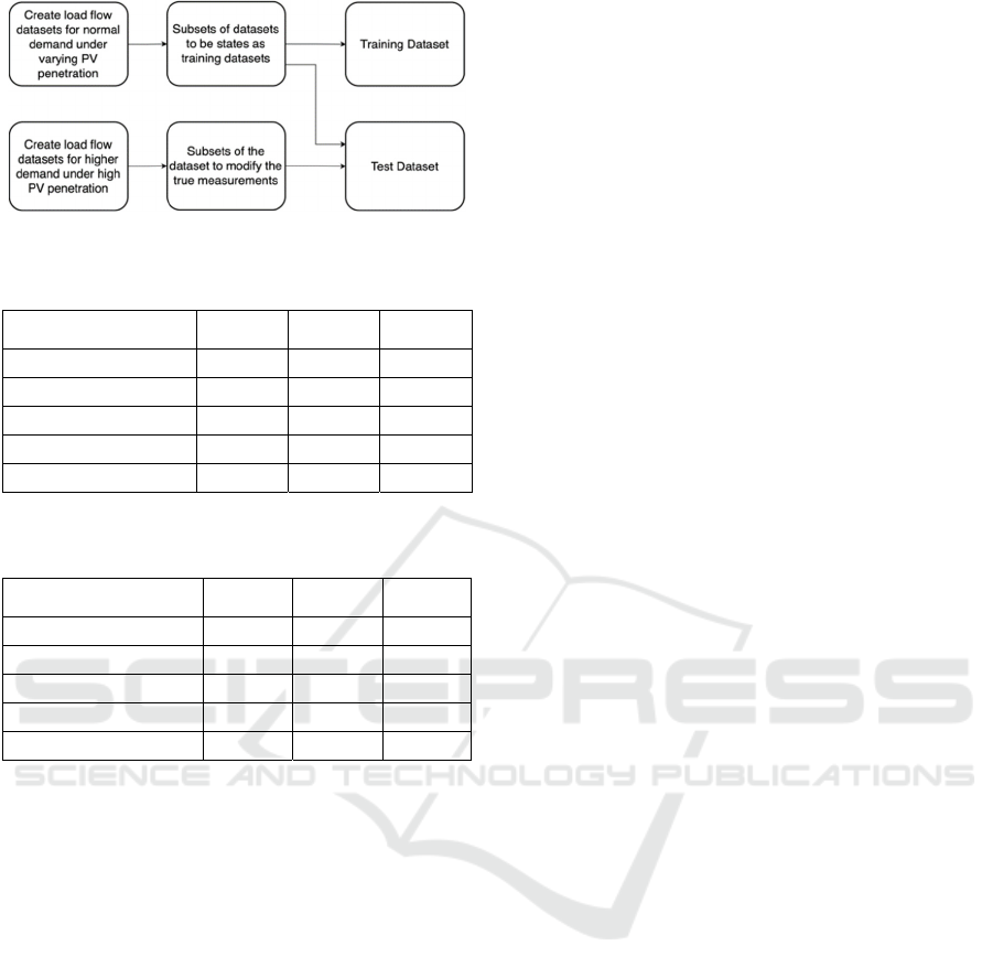
Figure 12: Machine learning training model.

Table 1: FDIA Detection Under 0% PV Penetration.

Algorithm Precision

False

Positive

False

Negative

Isolation Forest

93.9% 3% 13%

Local Outlier Factor

93.7% 2% 15%

OCSVM

96.3% 5% 9%

Mahalanobis Distance

93.9% 3% 13%

Kalman Filter

98.1% 1% 5%

Table 2: FDIA Detection Under Peak Load in 80% PV

Penetration.

Algorithm Precision

False

Positive

False

Negative

Isolation Forest

91.7% 4% 14%

Local Outlier Factor

91.7% 3% 15%

OCSVM

95.2% 5% 10%

Mahalanobis Distance

91.7% 3% 15%

Kalman Filter

68.5% 44% 5%

The machine learning algorithms are however not

100% efficient because the difference between the

characteristics of states during lower PV penetration

and mild false data injection attack is very subtle, and

we expect the results to improve with additional

training of the algorithms.

5 CONCLUSIONS

In this paper, we exposed a vulnerability associated

with model-based detectors and compared how

machine learning algorithms perform in the same

scenario. We concluded that the model-based detector

works best only on a grid environment with little to

no PV penetration. While dynamic thresholds can be

used to overcome this problem, we showed that the

grid’s behavior cannot be predicted accurately well

ahead of time. To attempt to do it accurately, massive

amounts of data from large number BTM devices

would have to be taken, which is not feasible now.

Finally, it was observed that, if trained substantially,

machine learning algorithms have the awareness to

understand if a degrading voltage profile is due to a

false data injection attack or a switch to PV

generators.

The paper used 5000 data points and 14 bus IEEE

setup for simulation. However, more accurate data

could be obtained if the simulation was done over

more load points that spanned a few days or even

weeks. Similarly, instead of using 14-bus, a larger

grid setup would have given a more realistic scenario.

These tasks could certainly be a done as future work

for the research. Additionally, new algorithms like

Artificial Neural Networks could be explored for this

research work.

REFERENCES

McDowell, J. & Walling, R. (2016, May 19). Reactive Power

Interconnection requirements for PV and wind plants:

Recommendations to NERC. UNT Digital Library

Till, J., You, S., Liu, Y., & Du, P. (2020). Impact of high PV

penetration on voltage stability. 2020 IEEE/PES

Transmission and Distribution Conference and

Exposition (T&D). https://doi.org/10.1109/td39804.2020

.9299973

Musleh, A. S., Chen, G., & Dong, Z. Y. (2020). A survey on

the detection algorithms for false data injection attacks in

smart grids. IEEE Transactions on Smart Grid, 11(3),

2218–2234. https://doi.org/10.1109/tsg.2019.2949998

Duan, J., Zeng, W., & Chow, M.-Y. (2018). Resilient

distributed DC optimal power flow against Data Integrity

Attack. IEEE Transactions on Smart Grid, 9(4), 3543–

3552. https://doi.org/10.1109/tsg.2016.2633943

Chung, H.-M., Li, W.-T., Yuen, C., Chung, W.-H., & Wen,

C.-K. (2017). Local cyber-physical attack with

leveraging detection in smart grid. 2017 IEEE

International Conference on Smart Grid

Communications (SmartGridComm). https://doi.org/

10.1109/smartgridcomm.2017.8340712

Inayat, U., Zia, M. F., Mahmood, S., Berghout, T., &

Benbouzid, M. (2022). Cybersecurity enhancement of

Smart Grid: Attacks, methods, and

prospects. Electronics, 11(23), 3854. https://doi.org/10.

3390/electronics11233854

Jiang, Q., Chen, H., Xie, L., & Wang, K. (2017). Real-time

detection of false data injection attack using residual

prewhitening in Smart Grid Network. 2017 IEEE

International Conference on Smart Grid

Communications (SmartGridComm). https://doi.org/

10.1109/smartgridcomm.2017.8340659

Kurt, M. N., Yilmaz, Y., & Wang, X. (2018). Distributed

quickest detection of cyber-attacks in Smart Grid. IEEE

Transactions on Information Forensics and

Security, 13(8), 2015–2030. https://doi.org/10.1109/

tifs.2018.2800908

Wang, X., Luo, X., Zhang, M., & Guan, X. (2019).

Distributed detection and isolation of false data

injection attacks in smart grids via nonlinear unknown

Exploring False Demand Attacks in Power Grids with High PV Penetration

133

input observers. International Journal of Electrical

Power & Energy Systems, 110, 208–222. https://

doi.org/10.1016/j.ijepes.2019.03.008

Karimipour, H., & Dinavahi, V. (2018). Robust massively

parallel dynamic state estimation of power systems

against Cyber-Attack. IEEE Access, 6, 2984–2995.

https://doi.org/10.1109/access.2017.2786584

Karimipour, H., & Dinavahi, V. (2017). On false data

injection attack against dynamic state estimation on

Smart Power Grids. 2017 IEEE International

Conference on Smart Energy Grid Engineering

(SEGE). https://doi.org/10.1109/sege.2017.8052831

Sahoo, S., Mishra, S., Peng, J. C.-H., & Dragicevic, T.

(2019). A stealth Cyber-Attack detection strategy for

DC microgrids. IEEE Transactions on Power

Electronics, 34(8), 8162–8174. https://doi.org/10.1109/

tpel.2018.2879886

Li, B., Ding, T., Huang, C., Zhao, J., Yang, Y., & Chen, Y.

(2019). Detecting false data injection attacks against

power system state estimation with fast go-

decomposition approach. IEEE Transactions on

Industrial Informatics, 15(5), 2892–2904. https://

doi.org/10.1109/tii.2018.2875529

Liu, L., Esmalifalak, M., Ding, Q., Emesih, V. A., & Han,

Z. (2014). Detecting false data injection attacks on

power grid by sparse optimization. IEEE Transactions

on Smart Grid, 5(2), 612–621. https://doi.org/

10.1109/tsg.2013.2284438

Ameli, A., Hooshyar, A., & El-Saadany, E. F. (2019).

Development of a cyber-resilient line current

differential relay. IEEE Transactions on Industrial

Informatics, 15(1), 305–318. https://doi.org/10.1109/

tii.2018.2831198

Ashok, A., Govindarasu, M., & Ajjarapu, V. (2016). Online

detection of stealthy false data injection attacks in

power system state estimation. IEEE Transactions on

Smart Grid, 1–1. https://doi.org/10.1109/tsg.2016.

2596298

Binna, S., Kuppannagari, S. R., Engel, D., & Prasanna, V.

K. (2018). Subset level detection of false data injection

attacks in smart grids. 2018 IEEE Conference on

Technologies for Sustainability (SusTech). https://

doi.org/10.1109/sustech.2018.8671357

Foroutan, S. A., & Salmasi, F. R. (2017). Detection of false

data injection attacks against state estimation in smart

grids based on a mixture gaussian distribution learning

method. IET Cyber-Physical Systems: Theory &

Applications, 2(4), 161–171. https://doi.org/10.1049/

iet-cps.2017.0013

Wang, D., Wang, X., Zhang, Y., & Jin, L. (2019). Detection

of power grid disturbances and cyber-attacks based on

machine learning. Journal of Information Security and

Applications, 46, 42–52. https://doi.org/10.1016/j.

jisa.2019.02.008

Zanetti, M., Jamhour, E., Pellenz, M., Penna, M.,

Zambenedetti, V., & Chueiri, I. (2019). A tunable fraud

detection system for advanced metering infrastructure

using short-lived patterns. IEEE Transactions on Smart

Grid, 10(1), 830–840. https://doi.org/10.1109/tsg.2017

.2753738

Viegas, J. L., & Vieira, S. M. (2017). Clustering-based

novelty detection to uncover electricity theft. 2017

IEEE International Conference on Fuzzy Systems

(FUZZ-IEEE). https://doi.org/10.1109/fuzz-ieee.2017.

8015546

Farsadi, Murtaza & Mohammadzadeh Shahir, Farzad &

Babaei, Ebrahim. (2017). Power System States

Estimations Using Kalman Filter.

Qi, J., Taha, A. F., & Wang, J. (2018). Comparing Kalman

filters and observers for power system dynamic state

estimation with model uncertainty and malicious cyber

attacks. IEEE Access, 6, 77155–77168. https://doi.org/

10.1109/access.2018.2876883

Taha, A. F., Qi, J., Wang, J., & Panchal, J. H. (2018). Risk

mitigation for dynamic state estimation against cyber

attacks and unknown inputs. IEEE Transactions on

Smart Grid, 9(2), 886–899. https://doi.org/10.1109/tsg.

2016.2570546

Minot, A., Sun, H., Nikovski, D., & Zhang, J. (2019).

Distributed estimation and detection of cyber-physical

attacks in Power Systems. 2019 IEEE International

Conference on Communications Workshops (ICC

Workshops). https://doi.org/10.1109/iccw.2019.8756653

Zhang, J., Welch, G., Bishop, G., & Huang, Z. (2014). A

two-stage Kalman filter approach for robust and real-

time power system state estimation. IEEE Transactions

on Sustainable Energy, 5(2), 629–636. https://

doi.org/10.1109/tste.2013.2280246

Manandhar, K., Cao, X., Hu, F., & Liu, Y. (2014).

Detection of faults and attacks including false data

injection attack in smart grid using Kalman filter. IEEE

Transactions on Control of Network Systems, 1(4),

370–379. https://doi.org/10.1109/tcns.2014.2357531

Zhang, J., Welch, G., & Bishop, G. (2010). Observability

and estimation uncertainty analysis for PMU placement

alternatives. North American Power Symposium 2010.

https://doi.org/10.1109/naps.2010.5618970

Mo, Yilin & Sinopoli, Bruno. (2010). False data injection

attacks in control systems. Preprints of the 1st Workshop

on Secure Control Systems.

Abur, A., & Expósito, G. A. (2004). Power System State

Estimation: Theory and implementation. CRC Press.

Reliable Energy Analytics. (2021). COMPARING ISO

LOAD FORECASTING METHODOLOGIES.

energycentral.com. https://energycentral.com/system/fi

les/ece/nodes/337915/2018-lf-methodologies-research-

report-final-ec.pdf

Wang, Y., Zhang, Z., Ma, J., & Jin, Q. (2022). KFRNN: An

effective false data injection attack detection in smart

grid based on Kalman filter and recurrent neural

network. IEEE Internet of Things Journal, 9(9), 6893–

6904. https://doi.org/10.1109/jiot.2021.3113900

Mokhtar, M., Robu, V., Flynn, D., Higgins, C., Whyte, J.,

Loughran, C., & Fulton, F. (2021). Prediction of

voltage distribution using deep learning and identified

key smart meter locations. Energy and AI, 6, 100103.

https://doi.org/10.1016/j.egyai.2021.100103

California ISO. (2022). CAISO. https://www.caiso.com

Labbe, R. R. (2020). Kalman and Bayesian Filters in

Python.

ICISSP 2023 - 9th International Conference on Information Systems Security and Privacy

134