Using Learned Indexes to Improve Time Series Indexing Performance on

Embedded Sensor Devices

David Ding, Ivan Carvalho and Ramon Lawrence

University of British Columbia, Kelowna, BC, Canada

Keywords:

Learned Indexing, Time Series, Database, Sensor Network, Embedded.

Abstract:

Efﬁciently querying data on embedded sensor and IoT devices is challenging given the very limited mem-

ory and CPU resources. With the increasing volumes of collected data, it is critical to process, ﬁlter, and

manipulate data on the edge devices where it is collected to improve efﬁciency and reduce network transmis-

sions. Existing embedded index structures do not adapt to the data distribution and characteristics. This paper

demonstrates how applying learned indexes that develop space efﬁcient summaries of the data can dramati-

cally improve the query performance and predictability. Learned indexes based on linear approximations can

reduce the query I/O by 50 to 90% and improve query throughput by a factor of 2 to 5, while only requiring a

few kilobytes of RAM. Experimental results on a variety of time series data sets demonstrate the advantages

of learned indexes that considerably improve over the state-of-the-art index algorithms.

1 INTRODUCTION

Embedded systems and IoT devices collect massive

amounts of data for use in environmental, industrial,

and monitoring applications. This time series data is

typically sent over the network to cloud servers for

processing. There is increasing focus on processing

data on the edge devices where it is collected to re-

duce network transmissions and power consumption.

There are multiple systems for indexing time se-

ries data on cloud servers (Wang et al., 2020; Yang

et al., 2019). These systems cannot be adapted to the

low-memory and CPU processing present on embed-

ded sensor devices. Specialized embedded indexes

such as Microhash (Zeinalipour-Yazti et al., 2005),

and sequential binary index for time series (SBITS)

(Fazackerley et al., 2021) demonstrate good index

performance with minimal memory usage. SBITS al-

lows for both querying by timestamp and data value.

Querying by timestamp is done using a linear inter-

polation search that outperforms binary search used

in prior embedded index methods.

Learned indexing is a technique for computing

models of the data distribution to efﬁciently predict

record locations. Various techniques have been used

including RadixSpline (Kipf et al., 2020) and the

Piece-wise Geometric Models (PGM) (Ferragina and

Vinciguerra, 2020). These indexes outperform tra-

ditional tree-based indexes for server applications.

There has been no prior work on adapting learned in-

dexes for embedded indexing.

The contribution of this work is the adaptation of

learned indexes for use with time series data collected

and processed by sensor devices. Learned indexing

techniques using RadixSpline and Piece-wise Geo-

metric Models are implemented and evaluated on ac-

tual sensor devices with real-world data sets. Experi-

mental results show a dramatic improvement of time

series query performance by a factor of two to ﬁve

times compared to binary search and linear interpo-

lation used by SBITS. With a small amount of index

memory, the query performance is signiﬁcantly im-

proved demonstrating that learned indexes are valu-

able for the sensor domain.

2 BACKGROUND

Indexing on ﬂash memory has unique characteristics,

and many index algorithms have been developed to

optimize performance (Fevgas et al., 2020). Index-

ing on sensor devices is typically on ﬂash memory

and requires additional optimizations beyond server-

based indexing. Data structures must adapt to the

unique performance characteristics of ﬂash mem-

ory such as different read and write times and the

erase-before-write constraint (i.e. no overwriting or

in-place writes). Common optimizations minimize

writes and use sequential rather than random writes.

A key consideration for sensor indexing is the lim-

ited resources. Devices have between 4 KB and 32

KB of SRAM memory, a processor running between

Ding, D., Carvalho, I. and Lawrence, R.

Using Learned Indexes to Improve Time Series Indexing Performance on Embedded Sensor Devices.

DOI: 10.5220/0011692900003399

In Proceedings of the 12th International Conference on Sensor Networks (SENSORNETS 2023), pages 23-31

ISBN: 978-989-758-635-4; ISSN: 2184-4380

 2023 by SCITEPRESS – Science and Technology Publications, Lda. Under CC license (CC BY-NC-ND 4.0)

16 and 128 MHz, and ﬂash storage consisting of a

SD card or raw ﬂash memory chips. Index structures

must minimize SRAM usage to be practical.

Data processing systems for embedded devices

such as Antelope (Tsiftes and Dunkels, 2011) and Lit-

tleD (Douglas and Lawrence, 2014) allow on-device

data processing. Improved query performance is

achievable by indexing the time series data. Ante-

lope (Tsiftes and Dunkels, 2011) supports an inline

index sorted by timestamp. Record lookup by times-

tamp is performed using binary search. MicroHash

(Zeinalipour-Yazti et al., 2005) also stores data as a

sorted time series data ﬁle and utilizes binary search

for timestamp queries. MicroHash uses range parti-

tioning to also index data values to support queries by

data value. PBFilter (Yin and Pucheral, 2012) uses

Bloom ﬁlters to summarize data for indexing. By se-

quentially writing the data and index ﬁles, PBFilter

outperforms tree and hashing techniques.

SBITS (Fazackerley et al., 2021) is a sequen-

tial indexing structure supporting timestamp and data

value based queries. Timestamp queries are efﬁ-

ciently done using linear interpolation. The location

of a record is predicted based on its timestamp and a

linear approximation of the data records stored. Given

that sensor data sets are often collected at consistent

intervals, location predication using linear interpola-

tion is highly effective and outperforms binary search.

Since data pages are ordered by timestamp, any times-

tamp can be retrieved in O(1) reads by calculating an

offset using the start timestamp, the query timestamp,

and the rate at which records are written to data ﬁle

(based on sampling rate and number of records per

block). The linear interpolation algorithm can be ex-

tended to support multiple different sensor sampling

rates and time periods by storing a linear approxima-

tion for each period, however that is not in the cur-

rent implementation. SBITS also supports efﬁcient

querying by data value by using a user-customizable

bitmap index. Prior experimentation (Ould-Khessal

et al., 2022) demonstrated that SBITS outperforms

MicroHash and other embedded indexing techniques.

Given the relative consistency of sensor timeseries

data, linear interpolation for location prediction is ef-

fective. However, there are cases in real-world data

sets where the data is not as regular and cannot be eas-

ily approximated by a single linear function. Events

such as changing the sampling frequency, power fail-

ures, or sensor outages may cause the data set to be

less than regular and index performance to degrade.

It is valuable to consider improved location predica-

tion techniques such as offered by learned indexes.

Learned indexes leverage machine learning mod-

els to outperform traditional indexes and were ini-

tially used for static, in-memory datasets (Kraska

et al., 2018). Early work on learned indexes fo-

cused on modeling the empirical Cumulative Distri-

bution Function (eCDF). Examples of such indexes

include the RMI (Kraska et al., 2018), RadixSpline

(Kipf et al., 2020), PGM Index (Ferragina and Vin-

ciguerra, 2020), and PLEX (Stoian et al., 2021).

The core idea of those learned indexes is the con-

nection between the eCDF and an element’s position

in a sorted array. Let P(A ≤ x) be the proportion

of elements smaller than a key x. Then, the posi-

tion of the key x in a sorted array with N elements

is pos = ⌊N · P(A ≤ x)⌋. Obtaining an exact formula

for P(A ≤ x) is challenging, hence the indexes opt to

train different kinds of machine learning models to

estimate the eCDF.

eCDF based learned indexes are highly effec-

tive for static, in-memory use cases. Marcus et al.

benchmarked the RMI, the PGM, and the RadixS-

pline against state-of-the-art traditional indexes on

real-world datasets (Marcus et al., 2020). Their ex-

perimental results show that the learned indexes al-

ways outperform traditional indexes on look-up time

and size, losing just on build time.

Although learned indexes are highly effective on

read-only workloads, adapting the indexes to handle

updates is a challenge. This is particularly relevant

for the sensor use case, as sensors are continually col-

lecting and indexing data. The index must handle a

continuous stream of appended data.

Learned indexes such as ALEX (Ding et al., 2020)

and LIPP (Wu et al., 2021) support updates. These in-

dexes are tree-based, and use the models to search the

tree. Instead of only approximating the eCDF, tree-

based learned indexes also focus on using the models

to partition the data evenly and achieve a small tree

height. The consequences of a smaller tree height are

faster lookups and a smaller memory footprint.

Despite the progress of updatable learned indexes,

they do not always beat traditional indexes in mixed

read-and-write scenarios. Wongkham et al. tested

ALEX, LIPP, and an updatable version of the PGM

in multiple scenarios in their benchmark (Wongkham

et al., 2022). Among their conclusions is that space

efﬁciency is not a guarantee of updatable learned in-

dexes. The gains in memory consumption are lowered

for ALEX and PGM under updates, and the LIPP con-

sumes more memory than traditional indexes. This

could potentially rule out applications of learned in-

dexes to sensors, as they are constantly updated and

have very limited memory resources.

SENSORNETS 2023 - 12th International Conference on Sensor Networks

3 ADAPTING LEARNED

INDEXES

Applying learned indexing structures for sensor time

series data requires supporting the continual increase

of the data size as new values are collected. There-

fore, we need to adapt learned indexes to support ap-

pend operations while keeping memory consumption

low. Further, learned indexes only apply to indexing

the sensor data by timestamp as records are stored

in a sorted ﬁle by timestamp as they are collected.

Learned indexes do not directly apply to indexing the

data (sensor values) in the record, which are not stored

in sorted order.

We focus on adapting bottom-up, eCDF based

learned indexes. Indexes that are built bottom-up such

as the RadixSpline do not require all the data in ad-

vance, in contrast to top-down modeling approaches

such as RMIs that require all data in advance and can-

not be easily deployed for the time series use case.

We adapt and deploy two structures for indexing: the

RadixSpline and the PGM Index.

The indexing approach is based on SBITS (Faza-

ckerley et al., 2021) and proceeds as follows:

• Each data record containing collected sensor val-

ues is stored in a buffered page in memory until

the page is full.

• A full data page is written to the sorted data ﬁle in

sequential order.

• After the page is written, an index record is cre-

ated storing the timestamp of the smallest record

on the data page and the data page index.

• The index algorithm must maintain its index

structure in memory with a bounded size (often

less than 1 KB) and may periodically ﬂush index

pages to storage for persistence.

Querying by timestamp is performed by using the

index. Querying by data value is unchanged from the

previous SBITS implementation as learned indexes

do not apply to the unsorted data values.

3.1 Piece-Wise Geometric Models

The Piece-wise Geometric Model index (PGM) is a

learned index that approximates the CDF via piece-

wise linear approximations (PLA) (Ferragina and

Vinciguerra, 2020). At the heart of the PGM lies a

hyperparemeter ε that controls the error bounds for

the linear approximations.

The original PGM index is built from the bottom-

up recursively. At the ﬁrst level, the PGM builds a

PLA over the set of points {(x

, i)}

i=0...n

using the op-

timal algorithm proposed by (O'Rourke, 1981) and

rediscovered by (Elmeleegy et al., 2009). For sub-

sequent levels, the PGM applies the same linear ap-

proximation strategy using the keys from the previous

level {(k

, j)}

j=0...s

as points for the PLA. The recur-

sion halts when there is a level with exactly one line.

We adapt the PGM by creating an append method

described in Algorithm 1. Notice that the method

does not know the number of levels for the PGM in

advance and starts by appending a key to the linear

approximation at the bottom level and propagating

the updates to the upper levels if necessary. Another

modiﬁcation of our implementation is the use of the

Swing Filter algorithm also proposed by (Elmeleegy

et al., 2009). The Swing Filter does not yield an opti-

mal number of lines, but requires only O (1) time and

memory to process a point. This is a beneﬁt in the

sensor use case, as the optimal Slide Filter requires

O(h) memory in its worst-case where h is the number

of points in the convex hull, which might not ﬁt in-

memory. Even though we adapted the PGM to sup-

port appends, its procedure for ﬁnding a key remains

unchanged from the original PGM (see Algorithm 2).

Algorithm 1: AppendPGMAdd(Pgm, x).

L ← pgm.countLevels();

K ← x;

for i ← 0 to L − 1 do

c ← pgm.levels[i].countPoints();

pgm.levels[i].add(K); // add

implements the Swing Filter

if pgm.levels[i].countPoints() > c then

K ← pgm.levels[i].getLastKey();

else

return;

/* If the algorithm reached this

step we need to create a new

level */

pgm.levels[L] = newPGMLevel();

ﬁrstK ← pgm.levels[L-1].getFirstKey();

lastK ← pgm.levels[L-1].getLastKey();

pgm.levels[L].add(ﬁrstK);

pgm.levels[L].add(lastK);

return;

3.2 RadixSpline

The RadixSpline is a learned index that approximates

the CDF via a linear spline and a radix table storing

spline points (Kipf et al., 2020). The two hyperpa-

rameters that shape the RadixSpline are ε, the error

bound for the spline approximation, and r, the size of

the preﬁx of the radix table entries.

The RadixSpline builds an error-bounded linear

Using Learned Indexes to Improve Time Series Indexing Performance on Embedded Sensor Devices

Algorithm 2: QueryAppendPGM(Pgm, x).

if x < pgm.levels[0].getFirstKey() then

return NotFound;

L ← pgm.countLevels();

m← 0; // index of the model at the

i-th level

for i ← L − 1 to 1 do

a ← pgm.levels[i].getSlope(m);

b ← pgm.levels[i].getIntercept(m);

pos ← ⌊a · x + b⌋;

lo ← max{0, pos − ε − 1};

hi ← min{pgm.levels[i].countKeys() −

1, pos + ε + 1};

m ← smallest value of j such that x ≥

pgm.levels[i-1].getKey(j) and

lo ≤ j ≤ hi;

a ← pgm.levels[0].getSlope(m);

b ← pgm.levels[0].getIntercept(m);

pos ← ⌊a · x + b⌋;

lo ← max{0, pos − ε − 1};

hi ← min{pos + ε +

1, pgm.levels[0].countKeys() − 1, };

/* Search is an implementation of

binary search or linear search

over the original array

containing the keys */

return Search(x, lo, hi);

spline over the empirical CDF using the greedy algo-

rithm proposed by (Neumann and Michel, 2008). Af-

ter the spline is built, the preﬁxes of the spline points

are inserted in a radix table. The radix table is a ﬂat

array of size 2

where each entry in the table maps to

a range in the spline.

Querying for a point in a RadixSpline is done in

three steps. The ﬁrst step is to look for the preﬁx of

the key being searched in the radix table, and ﬁnd the

corresponding spline point. Given the spline point,

calculate a narrow range of size 2ε where the key

could be using linear interpolation. The last step is to

ﬁnd the key in the range using linear or binary search,

which is a quick operation because 2ε is constant.

We adapted the RadixSpline to support appends

by implementing a streaming version of the GreedyS-

pline proposed in (Neumann and Michel, 2008), as

described in Algorithm 3. After appending a point,

we check if we can adjust the last spline segment to

correctly approximate the point position within ε. If

that is not the case, we create a new spline segment

covering the new point and propagate the new spline

point to the radix table (see Algorithm 4).

Algorithm 3: RadixSplineAdd(Rs, x).

c ← rs.spline.countPoints();

rs.spline.add(x); // Add implements

GreedySpline

if rs.spline.countPoints() > c then

K ← rs.spline.getLastKey();

RadixTableInsert(rs, K, c); // see

Algorithm 4

return;

Algorithm 4: RadixTableInsert(Rs, K, pos).

r ← rs.r; // radix prefix size

K ← K - rs.minKey;

nB ← mostSigniﬁcantBit(bitShiftRight(K,

rs.shiftSize)); // number of bits

required to fit on the table

∆ ← max(nB - r, 0); // difference

between the available and

required number of bits

if ∆ > 0 then

/* New key triggers table

rebuild with new prefix size

in order to fit; we merge the

old radix entries considering

the new bit shift */

rs.shiftSize ← rs.shiftSize + ∆;

newTable ← allocateTable( 2

);

for i ← 0 to 2

j ← bitShiftRight(i, ∆);

newTable[j] ← min(rs.table[i],

newTable[j]);

for i ← 2

r−∆

to 2

newTable[i] ← INT MAX;

rs.table ← newTable;

// Update entry of the radix table

with the new pos

T ← bitShiftRight(K, rs.preﬁxSize);

rs.table[T] ← min(rs.table[T], pos);

return;

4 EXPERIMENTAL RESULTS

The experiments evaluated sensor time series index-

ing for multiple real-world data sets. The sensor

hardware platform has a 32-bit Microchip ARM

Cortex

M0+ based SAMD21 processor with clock

speed of 48 MHz, 256 KB of ﬂash program mem-

ory and 32 KB of SRAM. The hardware board has

several different memory types including a SD card

SENSORNETS 2023 - 12th International Conference on Sensor Networks

and serial NOR DataFlash

which supports in-place

page level erase-before-write. This platform is repre-

sentative of embedded devices with commonly used

32-bit ARM processors. The serial NOR DataFlash

was used to test performance on raw memory without

a ﬂash translation layer (FTL). Testing on raw mem-

ory insures no overhead with FTL maintenance op-

erations and allows for the highest read performance.

Platform performance characteristics are in Table 1.

The experiments benchmark four indexes:

• Binary Search: A binary search over the sorted

data. This is the baseline for the benchmark and

requires no additional memory.

• SBITS: SBITS using linear interpolation requires

8 bytes to maintain linear approximation. SBITS

was optimized to default to binary search if its

predictions were off signiﬁcantly.

• PGM: A modiﬁed version of the PGM Index with

support for appends and error-bound of ε = 1.

• RadixSpline: A modiﬁed version of the RadixS-

pline with support for appends, error-bound set to

ε = 1 and radix preﬁx size of r = 0 that offered the

best performance with smallest memory usage.

The experiments measure four core metrics: the

query throughput, the number of I/Os per query,

memory consumption, and insertion throughput.

These metrics are relevant to common use cases of

sensors such as querying by timestamp and ingesting

new data. We report the average of the metrics based

on three separate runs. The real-world data sets eval-

uated are in Table 2. The data sets cover a variety of

sensor use cases including environmental monitoring,

smart watches, GPS phone data, and chemical con-

centration monitoring. The environmental data sets

sea and uwa were originally from (Zeinalipour-Yazti

et al., 2005) and have been used in several further

experimental comparisons (Fazackerley et al., 2021;

Ould-Khessal et al., 2022). We also present the eCDF

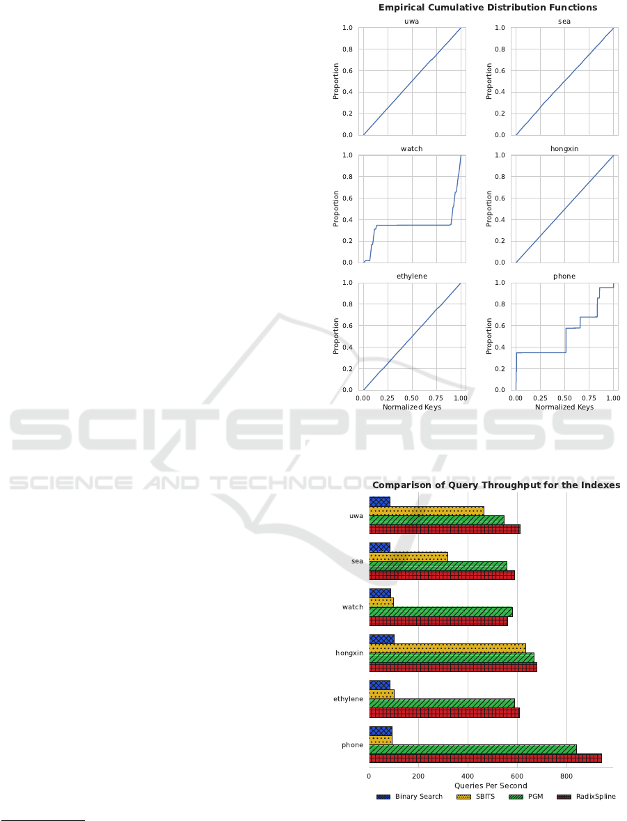
for the datasets in Figure 1.

4.1 Query Performance

One common use case of processing data in edge de-

vices is to query timestamps. We measure the query

throughput for searching timestamps. After the sen-

sor data was inserted, 10,000 random timestamp val-

ues were queried in the timestamp range. Data was

collected on the time to execute all queries and the

number of I/O operations performed.

https://www.dialog-semiconductor.com/products/

memory/dataﬂash-spi-memory

Figure 1: eCDFs for the experimental datasets. The PGM

and the RadixSpline use a collection of linear models to

approximate those with bounded-error of ε.

Figure 2: Average query throughput among the indexes for

each dataset in the benchmark. Higher rates indicate better

results. The RadixSpline and PGM consistently outperform

SBITS and binary search.

Using Learned Indexes to Improve Time Series Indexing Performance on Embedded Sensor Devices

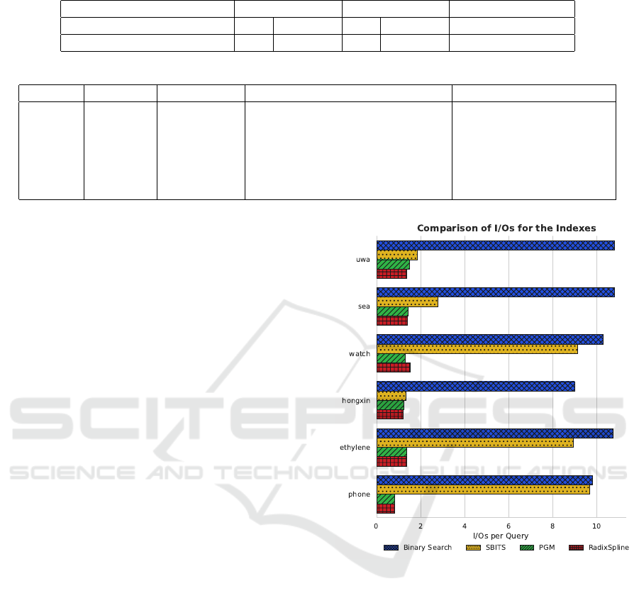
Table 1: Hardware Performance Characteristics.

Reads (KB/s) Writes (KB/s)

Seq Random Seq Random Write-Read Ratio

M0+ SAMD21 (DataFlash) 475 475 38 38 12.5

Table 2: Experimental Data Sets.

Name Points Points Used Sensor Data Source

sea 100,000 100,000 temp, humidity, wind, pressure SeaTac Airport

uwa 500,000 500,000 temp, humidity, wind, pressure ATG rooftop, U. of Wash.

hongxin 35,064 35,000 PM2.5, PM10, temp (Zhang et al., 2017)

ethylene 4,085,589 100,000 ethylene concentration (Fonollosa et al., 2015)

phone 18,354 18,000 smartphone X/Y/Z magnetic ﬁeld (Barsocchi et al., 2016)

watch 2,865,713 100,000 smartwatch X/Y/Z gyroscope (Stisen et al., 2015)

The query throughput results are in Figure 2. Ap-

plying learned indexes to sensor time series is very ef-

fective. The PGM and the RadixSpline always outper-

form SBITS with signiﬁcant improvements on highly

variable datasets.

For the hongxin and uwa datasets, the gains are

more modest ranging from 1.05x-1.20x for the PGM

and 1.06x-1.31x for the RadixSpline. These datasets

are highly linear such that an interpolation search

achieves its best-case scenario. Since the PGM and

RadixSpline use PLAs to model the dataset, they also

perform well just like the interpolation search.

However, datasets such as watch, ethylene, and

phone prove to be more challenging for SBITS. Its

performance is affected and becomes closer to the

throughput of the binary search baseline. Learned in-

dexes, on the other hand, extend their lead and stay

resilient to the change in data distribution. The per-

formance gains range from 1.8x-8.9x for the PGM

and 1.8x-10x for the RadixSpline. This indicates that

the learned indexes have more ﬂexible models that de-

scribe the data distribution better.

The query throughput difference between RadixS-

pline and PGM is within 10% for all data sets. Since

both approaches use linear approximations, the dif-

ference relates to how the linear approximations are

themselves indexed. For these experiments, the radix

table for RadixSpline was allocated no space, and

only a binary search was used on the spline points.

This is effective as there are very few points. Perfor-

mance testing with using a radix table of size r = 4

and r = 8 demonstrated no query performance beneﬁt

while consuming precious RAM. This makes sense

as the radix table is only saving a few comparisons

when searching the spline points in memory, and the

search time is dominated by the I/Os performed to

the ﬂash memory. PGM produces a multi-level in-

dex, which takes some more space and a little longer

to query. Overall, both approaches are effective and

Figure 3: Average number of I/Os per query among the in-

dexes for each dataset in the benchmark. Lower rates are

better. Learned indexes signiﬁcantly reduce the number of

required I/Os.

greatly improve on binary search or single linear in-

terpolation. The trade-off between the query perfor-

mance and memory space is discussed further in Sec-

tion 4.2.

Another relevant metric for querying is the num-

ber of I/Os per query. The number of I/Os per-

formed dominates the query response time and is es-

pecially important in embedded systems were pre-

dictable real-time performance is desirable. Figure 3

displays the average number of I/Os performed per

timestamp query. Binary search performs O(logN)

I/Os and has signiﬁcantly more I/Os than the other ap-

proaches. SBITS’ single linear interpolation is effec-

tive in many cases, however data sets like phone are

SENSORNETS 2023 - 12th International Conference on Sensor Networks

poorly approximated by one linear approximation and

the algorithm frequently defaults to binary search due

to poor prediction accuracy. Both PGM and RadixS-

pline have guaranteed error bounds in their construc-

tion. With ε = 1, at most 2 I/O are performed for any

lookup with the average often around 1.3 to 1.5. This

predictable performance is a major beneﬁt for using

these learned indexes.

4.2 Memory Space Efﬁciency

It is critical for learned indexes to have a small mem-

ory footprint in order to be useful for embedded sys-

tems. Many traditional techniques cannot be applied

to embedded systems because of the RAM constraints

(Fazackerley et al., 2021), which prompts adaptations

that trade memory and performance. The memory re-

sults are in Table 3.

Table 3: Memory consumption comparison among the

learned indexes for each dataset in the benchmark.

Memory Consumption (in KB)

PGM RadixSpline

uwa 0.04 0.09

sea 1.88 0.96

watch 7.80 2.43

hongxin 0.10 0.07

ethylene 0.40 0.12

phone 1.09 0.25

All indexes ﬁt in memory, with the maximum

amount of memory used being 7.80 KB. The results

indicate that the RadixSpline consumes less memory

than the PGM. This is to be expected, as both the

spline and the bottom level of the PGM contain a very

similar set of linear approximations. The key differ-

ence between the two is their approach to ﬁnding the

linear approximation to use. The RadixSpline uses a

small radix table to index spline points. The PGM

uses a recursive approach building additional PLAs.

Since the size of the table from the RadixSpline is

parametrized by r, it is possible to sacriﬁce a little

query performance to achieve less memory usage.

For our choice of r = 0, the difference in mem-

ory consumption is signiﬁcant, and the difference in

query performance is negligible as performance is

dominated by the number of I/Os not comparisons in

memory. The PGM uses two to four times the amount

of memory as the RadixSpline for ﬁve out of the six

datasets, with the exception being the easiest dataset

uwa.

By modifying the error bound (ε), both ap-

proaches can reduce their memory footprint at the

sacriﬁce of more query I/Os and lower query through-

put. Table 4 shows statistics on the index size in bytes,

I/Os performed per query, and query throughput in

queries/second for the sea data set for multiple differ-

ent values of ε. There is a quite signiﬁcant index size

reduction for increasing ε to 2 or 3. Even though the

I/Os per query increases, it is always bounded by ε.

This allows designers to determine the exact perfor-

mance trade-offs in terms of space and query I/Os in

a predictable fashion.

4.3 Insertion Performance

Adding indexes beneﬁts query performance, but they

can also impact the insertion time. It is critical for

sensors to keep ingesting data; hence the need to mon-

itor the insertion throughput to ensure they match the

sensors required sampling rate. For insertion perfor-

mance, the N records used for each data set were in-

serted at the maximum possible rate of the hardware.

The insertion performance is dominated by the I/Os

for writing the data pages to storage, but the index

construction time may have some overhead. The in-

sertion rates in Figure 4 show the maximum rates pos-

sible on the hardware for each data set and index.

The baseline for insertion performance is the bi-

nary search case which consists of a simple data

record append and no indexing overhead. The aver-

age throughput was 1967 inserts per second. Since

the incoming timestamps are strictly increasing and

because binary search does not store any additional

information to help on the search, this represents the

upper bound for insertion performance.

SBITS and RadixSpline were the indexes that had

the highest insertion throughputs at 1966 and 1965

inserts per second, respectively. They almost match

the scenario with no index at all. The results are

consistent with earlier experiments for SBITS (Ould-

Khessal et al., 2022), showing that the number of I/Os

to keep the index up to date is minimal. Perhaps the

most surprising result is for the RadixSpline, because

it needs to calculate spline points and update the radix

table. Our benchmark shows that the overhead for

these operations are small.

The PGM supports 1951 inserts per second, which

represents a less than 1% overhead. The PGM has

a slightly lower insert rate because some insertions

trigger changes on multiple levels of the PGM, while

RadixSpline triggers at most one change in the spline

and radix table. The PGM insertion throughput re-

mains competitive beating traditional embedded in-

dexes such as B-Trees (Ould-Khessal et al., 2022).

Using Learned Indexes to Improve Time Series Indexing Performance on Embedded Sensor Devices

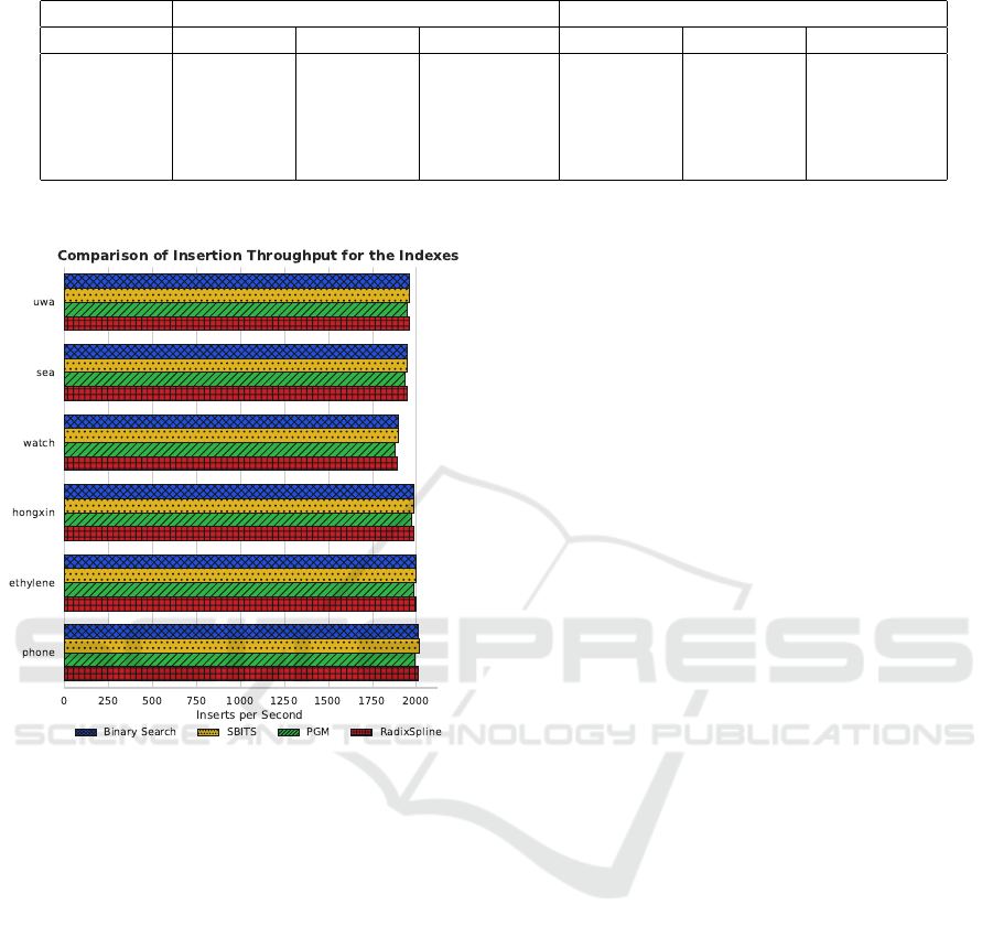
Table 4: Index Size in bytes, I/Os per Timestamp Query, and Query Throughput (queries/sec.) for Different Error Bounds ε.

RadixSpline PGM

Test Index Size Query I/O Throughput Index Size Query I/O Throughput

SEA ε = 1 932 1.40 588 1920 1.42 557

SEA ε = 2 436 1.85 461 856 1.91 440

SEA ε = 3 260 2.23 386 664 2.26 376

SEA ε = 5 212 3.12 281 496 3.41 256

SEA ε = 10 132 5.37 166 232 4.94 179

Figure 4: Average insertion throughput among the indexes

for each dataset in the benchmark. Higher rates indicate

better results. The insertion throughout is slightly lower for

the PGM, but overall learned indexes remain competitive.

4.4 Results Discussion

Overall, the experimental results demonstrate that

there are signiﬁcant advantages to using learned in-

dexes adapted for embedded time series data. The

most signiﬁcant advantage is the predictable and

bounded timestamp query performance. By specify-

ing a given error bound (ε), the maximum number of

I/Os per query is 2ε + 2. The query performance is

signiﬁcantly higher than SBITS linear interpolation

search or binary search. The overhead of the index in

terms of insertion throughput is minimal. To handle

the limited memory, the index size can be reduced by

increasing the error bound. In the experiments tested,

the index size was usually less than a few KB. The

index algorithms support real-time sensor data collec-

tion of almost 2000 records/second on the experimen-

tal hardware, which is signiﬁcantly above collection

rates for most applications.

5 CONCLUSIONS

This work adapted and applied learned indexes to

sensor time series data. Experiments indicate that

the RadixSpline and PGM are suitable to tackle the

challenge of indexing the amount of data embed-

ded systems collect under the unique constraints that

those systems have. This work is a bridge between

embedded system indexing and the original applica-

tions of learned indexing targeting large in-memory

databases. With the correct adaptations, it is possi-

ble to reuse these structures conceived to query large

static datasets and apply them in embedded systems

with tiny memory and frequent data appends.

Future work will extend learned indexes for sen-

sors to automatically handle hyperparameters and re-

quire less tuning. We envision learned indexes that

automatically adapt their parameters to ﬁt in the

limited resources in embedded systems, speciﬁcally

adapting the error bound to ensure the index ﬁts in

the memory available.

REFERENCES

Barsocchi, P., Crivello, A., Rosa, D. L., and Palumbo, F.

(2016). A multisource and multivariate dataset for in-

door localization methods based on WLAN and geo-

magnetic ﬁeld ﬁngerprinting. In 2016 International

Conference on Indoor Positioning and Indoor Navi-

gation (IPIN), pages 1–8. IEEE.

Ding, J., Minhas, U. F., Yu, J., Wang, C., Do, J., Li, Y.,

Zhang, H., Chandramouli, B., Gehrke, J., Kossmann,

D., Lomet, D., and Kraska, T. (2020). ALEX: An

updatable adaptive learned index. In Proceedings of

the 2020 ACM SIGMOD International Conference on

Management of Data, pages 969–984. ACM.

Douglas, G. and Lawrence, R. (2014). LittleD: a SQL

database for sensor nodes and embedded applications.

In Symposium on Applied Computing, pages 827–832.

Elmeleegy, H., Elmagarmid, A. K., Cecchet, E., Aref,

W. G., and Zwaenepoel, W. (2009). Online piece-wise

linear approximation of numerical streams with preci-

sion guarantees. Proc. VLDB Endow., 2(1):145–156.

Fazackerley, S., Ould-Khessal, N., and Lawrence, R.

SENSORNETS 2023 - 12th International Conference on Sensor Networks

(2021). Efﬁcient ﬂash indexing for time series data

on memory-constrained embedded sensor devices. In

Proceedings of the 10th International Conference on

Sensor Networks, SENSORNETS 2021, pages 92–99.

SCITEPRESS.

Ferragina, P. and Vinciguerra, G. (2020). The PGM-index:

a fully-dynamic compressed learned index with prov-

able worst-case bounds. PVLDB, 13(8):1162–1175.

Fevgas, A., Akritidis, L., Bozanis, P., and Manolopoulos,

Y. (2020). Indexing in ﬂash storage devices: a survey

on challenges, current approaches, and future trends.

VLDB J., 29(1):273–311.

Fonollosa, J., Sheik, S., Huerta, R., and Marco, S. (2015).

Reservoir computing compensates slow response of

chemosensor arrays exposed to fast varying gas con-

centrations in continuous monitoring. Sensors and Ac-

tuators B: Chemical, 215:618–629.

Kipf, A., Marcus, R., van Renen, A., Stoian, M., Kemper,

A., Kraska, T., and Neumann, T. (2020). RadixSpline:

a single-pass learned index. In Proceedings of the

Third International Workshop on Exploiting Artiﬁcial

Intelligence Techniques for Data Management, pages

1–5.

Kraska, T., Beutel, A., Chi, E. H., Dean, J., and Polyzotis,

N. (2018). The case for learned index structures. In

Proceedings of the 2018 SIGMOD International Con-

ference on Management of Data, pages 489–504.

Marcus, R., Kipf, A., van Renen, A., Stoian, M., Misra,

S., Kemper, A., Neumann, T., and Kraska, T. (2020).

Benchmarking learned indexes. Proc. VLDB Endow.,

14(1):1–13.

Neumann, T. and Michel, S. (2008). Smooth interpolating

histograms with error guarantees. In Lecture Notes

in Computer Science, pages 126–138. Springer Berlin

Heidelberg.

O'Rourke, J. (1981). An on-line algorithm for ﬁtting

straight lines between data ranges. Communications

of the ACM, 24(9):574–578.

Ould-Khessal, N., Fazackerley, S., and Lawrence, R.

(2022). Performance Evaluation of Embedded Time

Series Indexes Using Bitmaps, Partitioning, and

Trees. In Invited and revised papers of SENSORNETS

2021, volume 1674 of Sensor Networks, pages 125–

151. Springer.

Stisen, A., Blunck, H., Bhattacharya, S., Prentow, T. S.,

Kjærgaard, M. B., Dey, A., Sonne, T., and Jensen,

M. M. (2015). Smart devices are different: Assess-

ing and mitigating mobile sensing heterogeneities for

activity recognition. In Proceedings of the 13th ACM

Conference on Embedded Networked Sensor Systems,

SenSys ’15, page 127–140, New York, USA. ACM.

Stoian, M., Kipf, A., Marcus, R., and Kraska, T.

(2021). Towards practical learned indexing.

https://arxiv.org/abs/2108.05117.

Tsiftes, N. and Dunkels, A. (2011). A database in every

sensor. In Proceedings of the 9th ACM Conference

on Embedded Networked Sensor Systems, SenSys ’11,

page 316–332, New York, NY, USA. ACM.

Wang, C., Huang, X., Qiao, J., Jiang, T., Rui, L., Zhang,

J., Kang, R., Feinauer, J., Mcgrail, K., Wang, P., Luo,

D., Yuan, J., Wang, J., and Sun, J. (2020). Apache

IoTDB: Time-series database for Internet of Things.

Proc. VLDB Endow., 13(12):2901–2904.

Wongkham, C., Lu, B., Liu, C., Zhong, Z., Lo, E., and

Wang, T. (2022). Are updatable learned indexes

ready? Proceedings of the VLDB Endowment,

15(11):3004–3017.

Wu, J., Zhang, Y., Chen, S., Wang, J., Chen, Y., and Xing,

C. (2021). Updatable learned index with precise posi-

tions. Proc. VLDB Endow., 14(8):1276–1288.

Yang, Y., Cao, Q., and Jiang, H. (2019). EdgeDB: An

Efﬁcient Time-Series Database for Edge Computing.

IEEE Access, 7:142295–142307.

Yin, S. and Pucheral, P. (2012). PBFilter: A ﬂash-based

indexing scheme for embedded systems. Information

Systems, 37(7):634 – 653.

Zeinalipour-Yazti, D., Lin, S., Kalogeraki, V., Gunopulos,

D., and Najjar, W. (2005). MicroHash: An Efﬁcient

Index Structure for Flash-Based Sensor Devices. In

Proceedings of the FAST ’05 Conference on File and

Storage Technologies, pages 31–43. USENIX Associ-

ation.

Zhang, S., Guo, B., Dong, A., He, J., Xu, Z., and Chen,

S. X. (2017). Cautionary tales on air-quality improve-

ment in Beijing. Proceedings of the Royal Society

A: Mathematical, Physical and Engineering Sciences,

473(2205):20170457.

Using Learned Indexes to Improve Time Series Indexing Performance on Embedded Sensor Devices