DT-ML: Drug-Target Metric Learning

Domonkos Pog

any

and P

eter Antal

Department of Measurement and Information Systems, Budapest University of Technology and Economics,

Budapest, Hungary

Keywords:

Drug-Target Interaction Prediction, Drug Repositioning, Representation Learning, Metric Learning, Joint

Embedding Models, Negative Sampling.

Abstract:

The challenges of modern drug discovery motivate the use of machine learning-based methods, such as pre-

dicting drug-target interactions or novel indications for already approved drugs to speed up the early discovery

or repositioning process. Publication bias has resulted in a shortage of known negative data points in large-

scale repositioning datasets. However, training a good predictor requires both positive and negative samples.

The problem of negative sampling has also recently been addressed in subﬁelds of machine learning with

utmost importance, namely in representation and metric learning. Although these novel negative sampling

approaches proved to be efﬁcient solutions for learning from imbalanced data sets, they have not yet been

used in repositioning in such a way that the learned similarities give the predicted interactions.

In this paper, we adapt representation learning-inspired methods in pairwise drug-target/drug-disease predic-

tors and propose a modiﬁcation to one of the loss functions to better manage the uncertainty of negative

samples. We evaluate the methods using benchmark drug discovery and repositioning data sets. Results indi-

cate that interaction prediction with metric learning is superior to previous approaches in highly imbalanced

scenarios, such as drug repositioning.

1 INTRODUCTION

One of the main motivations for modern drug devel-

opment is the discovery of new candidate compounds

which can be used as medication. Developing a new

drug molecule is a long and expensive process; bring-

ing a new drug to market takes approximately 10–15

years and 1.5–2.0 billion USD (Wouters et al., 2020).

One possible way to accelerate the development pro-

cess is via drug repositioning. Repositioning or re-

purposing refers to using a known drug in a new ther-

apeutic application, which is a promising approach,

considered less time-intensive, costly, and risky com-

pared to de novo molecule design.

The different stages of drug development have

been heavily inﬂuenced by the rise of artiﬁcial in-

telligence technologies in recent years. As a result

of this, classical machine learning methods have be-

come increasingly common among drug-target inter-

action (DTI) prediction approaches (Bagherian et al.,

2021). We can reduce the cost and time required for

measuring the interactions with their help. Besides,

https://orcid.org/0000-0003-4968-7504

https://orcid.org/0000-0002-4370-2198

these models can later be used to estimate the inter-

action between an unknown protein and molecule, to

search for candidates at the beginning of the devel-

opment process that binds to a speciﬁc protein, or to

reveal a new therapeutic application to a known drug,

i.e., repositioning (Harrer et al., 2019).

The simplest methods give estimates based only on

the similarity of molecules (Lee et al., 2016), or treat

the problem as a classiﬁcation and apply neural net-

works (Arany et al., 2022). Utilizing matrix factoriza-

tion (MF) is a common approach too (Bolg

ar and An-

tal, 2017). Still, most of the state-of-the-art (SOTA)

solutions use a general version of MF, namely pair-

wise

neural networks, such as the DeepDTA (

Ozt

urk

et al., 2018) or the AI-Bind (Chatterjee et al., 2021).

While the AI-Bind method utilizes pre-trained repre-

sentations, the DeepDTA model uses convolutional

encoders to transform the SMILES representations

from the molecular side and the amino acid sequences

from the protein side, thus providing the latent em-

beddings. These are concatenated, and a multilayer

perceptron (MLP) predicts the interactions. Most

Pairwise predictors have dual inputs, for instance, a

molecule and a protein, hence their name.

204

Pogány, D. and Antal, P.

DT-ML: Drug-Target Metric Learning.

DOI: 10.5220/0011691100003414

In Proceedings of the 16th International Joint Conference on Biomedical Engineering Systems and Technologies (BIOSTEC 2023) - Volume 3: BIOINFORMATICS, pages 204-211

ISBN: 978-989-758-631-6; ISSN: 2184-4305

 2023 by SCITEPRESS – Science and Technology Publications, Lda. Under CC license (CC BY-NC-ND 4.0)

of the aforementioned approaches were ﬁrst applied

in recommendation systems but are now considered

SOTA in the ﬁeld of DTI prediction too.

In repositioning, the aim is not to estimate a speciﬁc

interaction accurately but to establish a good disease

or molecule ordering. Accordingly, several methods

diverge from the traditional approach of treating in-

teraction prediction as a binary classiﬁcation and ap-

plying new loss functions better suited for ranking,

such as the Bayesian Personalized Ranking (BPR)

loss (Peska et al., 2017), also adopted from the ﬁeld

of recommendation systems.

Sufﬁcient quality and quantity of data are necessary

to apply a statistical learning approach. There are

plenty of available data sets for DTI prediction tasks,

but due to the high cost of interaction measurements,

the sparsity of these sets is relatively high. Moreover,

the number of known negative entries in drug-disease

interactions is lower than expected due to publica-

tion bias, where negative results are often not pub-

lished (Luo et al., 2021). Therefore, drug-disease

matrices are not only sparse, but often only the posi-

tive entries are known. This is a common problem in

repositioning tasks since SOTA predictors work with

a loss function such as binary cross-entropy (BCE),

which needs the negative samples too. One possible

solution is negative sampling, but since the unknown

entries can be either positive or negative, constructing

a proper sampling method is challenging.

The problem of unknown negative samples has

arisen in representation and (distance) metric learn-

ing too, especially in the ﬁeld of contrastive learn-

ing (Le-Khac et al., 2020). The main motivation is

to handle a large amount of available unlabeled data

with machine learning. One way to do this is to learn

representations in a self-supervised way. These em-

beddings can later be used in various supervised tasks

if they correctly capture the underlying data distribu-

tion.

Contrastive representation learning is one of the ﬁrst

widely used solutions, both in the computer vision,

natural language processing, and audio processing

domains (Le-Khac et al., 2020). Architecturally, these

methods can also be classiﬁed as pairwise, or rather,

joint embedding methods, because in most cases, one

input pair or triplet is compared at a time. The input

embeddings are ﬁrst processed by an encoder, thus

creating the latent/metric representations, which are

compared with a similarity function, and ﬁnally, a

loss function is used to optimize the similarity be-

tween the pairs. The similarities of positive and neg-

ative pairs are maximized and minimized during op-

timization. Positive pairs can easily be produced with

augmentation, but negative sampling is a challeng-

ing research problem. Unfortunately, using only pos-

itive pairs may lead to a collapse of the representation

space since providing the same embedding for all en-

tries can reduce the loss to zero. Therefore, negative

sampling is necessary for contrastive methods.

Over the last few years, the development of different

contrastive and, later, non-contrastive approaches has

been an area of particular research interest.

The ﬁrst approaches were the energy-based con-

trastive loss functions, such as the Pair loss (Hadsell

et al., 2006) and the Triplet loss (Collobert and We-

ston, 2008). They aim to associate low energy, i.e.,

low distance, to positive pairs and high energy to neg-

ative pairs.

A new, more effective family of methods is the proba-

bilistic loss functions. Here, a likelihood is described

by a SoftMax function with the similarity to the posi-

tive pair in the denominator and the similarity to all

positive and all negative samples in the numerator.

As opposed to the energy-based methods, it is not the

quality but the quantity of the selected negative sam-

ples that matters since we want to approximate the

denominator as accurately as possible. Therefore, we

often take the samples not only from a single batch

but keep their elements in a so-called memory bank

over several batches. One way of sampling is using

noise contrastive estimation (NCE), and a commonly

used probabilistic loss function is the infoNCE or also

known as normalized-temperature cross-entropy (NT-

Xent) (Chen et al., 2020). A modiﬁed version of

NT-Xent is called Supervised contrastive loss (Sup-

Con) (Khosla et al., 2020). The authors of this paper

performed supervised representation learning, where

the labels resulted from a classiﬁcation problem, and

proposed SupCon, which can handle entities belong-

ing to the same class. Another function is the cir-

cle loss (Sun et al., 2020). The novelty is that it

does not increase the similarity of positive pairs and

decrease the similarity of negative pairs equally but

adaptively assigns different gradient weights. It does

this by deﬁning an optimum for the positive and neg-

ative similarities and then weighting each pair by the

deviation from it.

Because of the efﬁciency problems associated with

negative sampling, research in recent years has fo-

cused on non-contrastive approaches, which also aim

to avoid latent collapse but do so without nega-

tive samples, for instance, the Variance-Invariance-

Covariance Regularization, (VICReg) (Bardes et al.,

2021).

There are striking similarities between pairwise

DTI prediction methods and joint embedding repre-

sentation learning approaches. Namely, both utilize

two inputs, from which two latent embeddings are

DT-ML: Drug-Target Metric Learning

205

learned, and the output is given by comparing them.

For example, the concatenation and MLP, mentioned

by the DeepDTA and AI-Bind models, can be consid-

ered a special similarity function with trainable pa-

rameters.

This analogy is also true for the MF approaches,

where the similarity function is a simple dot prod-

uct. In the Metric Factorization (Zhang et al., 2018)

collaborative ﬁltering method, the idea appeared that

during matrix factorization, we map users and prod-

ucts into a common space, and the similarity in this

space is the prediction. But this was exploited only

to the extent that instead of scalar multiplication, Eu-

clidean distance was used. The ﬁrst successful ap-

proach that combines the two is called Collaborative

Metric Learning (CML) (Hsieh et al., 2017), which

uses the Weighted Approximate-Rank Pairwise Loss

(WARP) (Weston et al., 2010). The loss uses triplets

of a user and a positive and negative item and gives

weights to the triplets proportional to the approxi-

mated rank of the positive sampled item in the row

of the given user, i.e., those who are further back in

the row are penalized more. This way, the WARP is

better suited for ranking than the BCE loss, the au-

thors have also tried the BPR ranking-based loss, but

the WARP was found to be superior.

To the best of our knowledge, novel negative sam-

pling solutions developed in the ﬁeld of metric learn-

ing have not yet been applied to drug repositioning

or DTI prediction this way, namely by treating the

learned similarity as a predicted interaction. How-

ever, we have seen that ideas that have worked in the

collaborative learning ﬁeld are adopted sooner or later

by interaction prediction methods. This would be par-

ticularly useful for drug repositioning because metric

learning-based approaches provide better solutions to

the problem of negative samples than the current re-

purposing methods, mainly using BCE loss with neg-

ative sampling. Some approaches use BPR, which is

better suited for ranking, but the novel contrastive and

non-contrastive loss functions have not yet been uti-

lized to predict interactions. In current approaches,

representation learning is only used in the pre-training

phase, e.g., to learn node representations on a multi-

modal, heterogeneous knowledge graph. Later these

embeddings are concatenated and used in interaction

prediction tasks with a BCE loss function (Li et al.,

2022), or the adjacency matrix is reconstructed from

them (Chen et al., 2022).

To this end, we propose a drug-Target Metric

Learning (DT-ML) approach that combines the two

methods. In this paper, different metric learning-

based methods are utilized and examined by their ap-

plicability to interaction prediction and drug reposi-

tioning. According to the results, among the various

DT-ML approaches compared, the ones using proba-

bilistic loss functions have proven superior, even bet-

ter than the current SOTA. Additionally, we propose

modifying one of the used loss functions, which could

further improve the results.

2 METHODOLOGY

An overview of the DT-ML methodology is shown in

Figure 1, detailing the data sets, architecture, similar-

ity and loss functions, and metrics used in the evalua-

tion.

2.1 Data and Representations

We utilized two widely used benchmark data sets to

evaluate our models, namely KiBA (Tang et al., 2014)

and ChEMBL (Gaulton et al., 2017). The former is

a DTI data set, with interactions between molecules

and proteins and known negative entries; the latter is

used for repositioning, as it contains drugs with only

positive indications of human conditions, i.e., associ-

ated diseases. In addition, a third data set was used

to produce disease representations, namely the Dis-

GeNET (Pi

nero et al., 2016), which contains relation-

ships between diseases and genes.

The KiBA set contains 467 kinase proteins, and

their interactions with molecules are given with a

dissociation constant (pK

). After preprocessing

the compounds, we retained only those for which

the canonical SMILES descriptor is known, unique,

and contains no more than 100 non-hydrogen atoms,

yielding 50,418 molecules. We discretized the inter-

action data with a threshold of pK

= 3, as suggested

by the authors of DeepDTA. This resulted in 72,944

positive and 162,681 negative entries; thus, the den-

sity of the interaction matrix is ∼1%.

Among the many tried protein representations, the

512-dimensional CPCProt (Lu et al., 2020) proved to

be the best. On the compound side, the pretrained,

300-dimensional Mol2vec embedding (Jaeger et al.,

2018) gave the best results and was also the most efﬁ-

cient to work with, thus was chosen for all subsequent

work

Another data set we used is ChEMBL. It contains

drug-like bioactive substances that are already FDA-

approved or are in clinical trials, and associated in-

dications as Medical Subject Headings (MeSH) (Lip-

scomb, 2000). MeSH is a controlled vocabulary of

Utilizing Mol2vec on the input is widespread in the

literature, e.g., the AI-Bind model also uses it.

BIOINFORMATICS 2023 - 14th International Conference on Bioinformatics Models, Methods and Algorithms

206

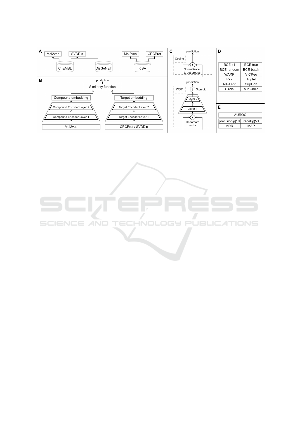
Figure 1: Visual summarization of the DT-ML methodology. (A) Used data sets with different types of molecule, protein, and

disease embeddings. (B) The implemented pairwise architecture. (C) Two used similarity functions in detail. (D) The list of

used loss functions and evaluation metrics (E).

life science concepts and terms also used in the litera-

ture. The part of the data set we use has 21,042 known

positive relationships between 4,755 drugs and 1,168

diseases, resulting in a density of 0.3789%.

To represent molecules, we used the Mol2vec. To ob-

tain disease embeddings, we utilized the DisGeNET

data set, which contains 1,134,924 positive entries

between 30,170 diseases and 21,666 genes, giving

a density of 0.1736%. Although there are no well-

established methods for representing diseases as there

are for proteins, a simple disease embedding can be

easily obtained in a semi-supervised way based on

the known disease-gene associations. We used trun-

cated singular value decomposition (SVD) to con-

vert the 21.666-dimensional sparse vectors into 64-

dimensional dense, gene-based disease representa-

tions, later referred to as SVDDis. MeSH concepts

map diseases from each column in the ChEMBL ma-

trix to a row in DisGeNET, thus we can use SVDDis

embeddings to represent diseases in the repositioning

data set. Another possible option is to use one-hot

representations, but this gave worse results, and with-

out the embeddings, the model is no longer able to

give predictions for new diseases.

2.2 Pairwise DTI Predictor

After preprocessing the data, we implemented a pair-

wise model using the PyTorch package.

We used the previously mentioned Mol2vec,

CPCProt, and SVDDis embeddings as inputs. Af-

ter scaling them on the training data, these embed-

dings are further transformed by two encoders, thus

creating latent representations. We concluded that

the method is less sensitive to the hyperparameters

of the encoders. After trying several combinations,

we ﬁnally chose two-layer MLP modules, with 512-

dimensional hidden, and 256-dimensional output lay-

ers. Between layers, a Rectiﬁed Linear Unit (ReLU)

activation and 20% dropout rate were used.

We deﬁned ﬁxed and trainable similarity functions

to obtain a prediction of a given interaction from the

metric embeddings and to measure the similarity be-

tween the entities. As a ﬁxed similarity, we have tried

Manhattan, Euclidean, mean squared, dot product,

and cosine similarities, among them, the latter proved

to be superior. Several trainable similarity functions

were tested too. We found that instead of concatena-

tion, it is better to take the Hadamard product and use

an MLP module with a sigmoid activation to obtain

the predictions. We used a multilayer perceptron with

two, 256, and 128-dimensional hidden layers and a

dropout with a rate of 10%. We refer to this later as

the weighted dot product (WDP) similarity.

Figure 1 shows the architecture of the pairwise

model and the used similarity functions. The model

can be used with BCE loss function as a simple pair-

wise DTI predictor, or even with different loss func-

tions according to the DT-ML approach.

2.3 Loss Functions

In our study, we tested several loss functions and neg-

ative sampling strategies.

As a ranking-based baseline, we implemented the

WARP and used it with a margin of 0.1.

In the other baseline approaches, we have used BCE

loss with sampling. The simplest approach is random

sampling, in this case, we tried different ratios, but we

found it best to sample twice as many negative sam-

ples as the number of known positives. This approach

is later referred to as BCE random.

DT-ML: Drug-Target Metric Learning

207

We tested the closed-world assumption, where all the

unknown entries are assumed to be negative, in this

case, the models worked with a fully completed ma-

trix. We refer to this as BCE all.

This method is inefﬁcient to use on the KiBA data

set due to the number of possible interactions. On the

other hand, in the KiBA data set, there are known neg-

ative interactions too, which can be utilized instead of

sampling. In most cases, we discarded the negative

entries of the KiBA set and used negative sampling

just as with the ChEMBL data set so as not to com-

promise comparability, but we kept one case where

we used the known negatives (BCE true).

We have also examined sampling during training,

here, negative samples were given by unknown sam-

ples within a batch (BCE batch).

To improve the results, we weighted the positive and

negative terms in the BCE loss. The weights are in-

versely proportional to the proportion of positive and

negative samples in the data set. So even though there

are more negative samples, they are taken into ac-

count with less weight, this way, we can express the

uncertainty in the noisy negative sampling.

The above-listed baseline approaches represent

the current SOTA, which we compared with several

metric learning-inspired loss functions. Compared to

the previous BCE and WARP functions, one of the

main differences is that DT-ML methods are not only

able to compare molecules with targets, but they also

utilize molecule-molecule and target-target similari-

ties in a semi-supervised way. This way, molecules,

and targets are represented in a common latent space,

and here the same similarity function is applied to

compare the different types of modalities with them-

selves and with each other

. During the optimization

of the DT-ML models, only the interacting molecule-

target pairs within a batch are considered positive,

negative pairs are sampled from the various possible

molecule-molecule, molecule-target, and target-target

combinations.

We have tried all loss functions implemented in

the PyTorch Metric Learning framework (Musgrave

et al., 2020). Of the several ﬁxed and learnable simi-

larity functions we tried, cosine proved to be the best

for these approaches.

First, we examined energy-based loss functions, such

as pair and triplet loss. We used them with a margin

of 0.2, which we found to be optimal. The quality

of the negative samples is a signiﬁcant factor in using

energy-based functions, hence it is important to select

One possible hypothesis is that these embeddings carry

information about binding sites, individuals that share a

common or related binding site will be close in the latent

space.

useful samples. With triplet loss, we only use triplets

in which the positive pair has a greater similarity than

the negative, but the difference between them is less

than the predeﬁned margin.

Among the tested probabilistic loss functions, NT-

Xent, SupCon, and Circle losses were in the top three.

For NT-Xent, a temperature hyperparameter of 0.01

was found to be optimal, and a memory bank capa-

ble of containing 512 interactions was used to fur-

ther improve performance. SupCon can handle en-

tities belonging to the same class better than previous

loss functions. Indeed, when considering molecules

as classes, we obtained better results. This means

that targets binding to the same compound are form-

ing positive pairs in the given batch

. The tempera-

ture parameter was set to 0.01 for SupCon too. The

best results were obtained with the Circle loss func-

tion. Besides the γ temperature hyperparameter, it has

two optima and two margins for the positive and neg-

ative pairs, but for simplicity, the authors have used

only one m hyperparameter to deﬁne them. Over the

various investigated combinations, m = 0.4, γ = 40

proved to be optimal. Because of the uncertainty of

the negative samples, we propose a modiﬁed version

where the positive and negative samples have sepa-

rate hyperparameters, m

and m

, respectively. With

our Circle loss function, we gave negative samples

a softer margin parameter of m

= 0.6, and positive

samples a harder margin of m

= 0.3, this way, we

were able to achieve further improvements.

Finally, we examined methods that do not require

negative sampling at all, such as VICReg. This

worked best when the weights of the variance, invari-

ance, and covariance loss terms were equal.

2.4 Evaluation Methods

To evaluate the approaches mentioned above, we uti-

lized a row-wise train-test split with 5-fold cross-

validation. This way, the test data matrix contains

only rows/molecules which were not included during

training, but all the columns/targets used in the evalu-

ation were seen in the training data too. We used ﬁve

metrics in total to compare the various methods.

One of them is the area under the receiver op-

erating characteristic curve (AUROC), which is fre-

quently used to evaluate binary classiﬁcation tasks,

The intuition behind this is the previously mentioned

binding site analogy, as a protein or the proteins associated

with one disease contain – on average – far more binding

sites than the number of molecule substructures matching

different sites. Thus, there is a high probability that proteins

that share binding molecules will have a common binding

site, so their representations should be similar indeed.

BIOINFORMATICS 2023 - 14th International Conference on Bioinformatics Models, Methods and Algorithms

208

hence widespread in interaction prediction too. It

only makes sense to use this metric with the KiBA

data set, because the ChEMBL does not have any

known negative entries. We calculated the AUROC

values on the test columns, which had at least 50 pos-

itive and 50 negative entries in the whole KiBA data

set, after that we took the column-wise average.

We also used four ranking-based metrics because,

in repositioning, the order of the predicted interac-

tions matters more than the actual predicted values of

the interactions. To this end, we calculated the aver-

age precision@10 (later referred to as PREC) of rows

in which there were at least ten entries among the test

set, and the mean recall@50 (REC) value over rows

in which there were at least 5 entries. We also used

the Mean Reciprocal Rank (MRR) and the Mean Av-

erage Precision (MAP).

These values were calculated both at row and col-

umn levels. This was necessary, because, on one

hand, most often, we are not looking for diseases for

a known drug, but rather vice versa, and on the other

hand, this way we can better detect overﬁtting.

3 RESULTS

We ran our models on a 32GB NVIDIA Tesla

V100 GPU. Among the optimization algorithms tried,

Adaptive Moment Estimation (Adam) proved to be

the best, using an L2 weight decay with a weight

of 10

−5

and a learning rate of 5 ∗ 10

−5

. After a

Xavier weight initialization, we trained the models

over 24 epochs in the case of the KiBA, and over 128

epochs in the case of the ChEMBL data set, we used

a batch size of 256 in both cases. Finally, we evalu-

ated the aforementioned approaches according to the

classiﬁcation-based and the four ranking-based met-

rics.

On the KiBA data set, according to the AUROC

metric, the SOTA BCE true approach outstandingly

outperformed all the other methods, which is not sur-

prising, since it is the only one using the known pos-

itive and negative entries as well. With the WDP and

Cosine similarities, it managed to reach 0.7851 and

0.7391 AUROC respectively, which are the highest

achieved values among all methods for both similar-

ity functions.

Considering the ranking-based metrics, the results

on the KiBA data set are shown in table 1 while the

results on the ChEMBL set can be seen in table 2.

Although BCE loss trained on the known negatives

is still the most suitable for classiﬁcation, some of

the DT-ML approaches perform better for reposition-

ing

. Among them, the energy-based and the non-

contrastive loss functions achieve poor scores, while

the probabilistic methods perform particularly well,

even better than the SOTA.

The column-based metrics are lower on average

because there are much more rows than columns in

the test data. However, these metrics are more rel-

evant, as they can detect overﬁtting due to the row-

wise train-test split. SOTA approaches using BCE

or WARP loss reach great results in some of the

row-based metrics but perform poorly according to

column-wise evaluation. In the case of WARP, one

possible reason other than the row-wise split is that

it only uses row-wise ranking, thus attending mainly

to the column representations. This way, interactions

with the same target got similar predictions, which is

not a problem considering row-wise evaluation, but

the model is not able to distinguish interactions be-

tween a given target and different molecules. How-

ever, with DT-ML methods, this inequality between

row-, and column-wise evaluations does not apply.

It can be concluded that DT-ML approaches, es-

pecially the ones with a probabilistic loss function,

perform well at both row and column levels. Mostly

column-wise ranking metrics should be considered

when selecting an appropriate method for drug repo-

sitioning, and according to them, Circle loss, or our

modiﬁed version of it, performs best.

4 CONCLUSIONS

We have seen the challenges inherent in drug discov-

ery and how deep learning-based interaction predic-

tion and repositioning, can accelerate the develop-

ment process. Most of the SOTA repositioning ap-

proaches utilize a DTI predictor, which needs both

positive and negative entries to train. However, neg-

ative results are often not published, thus there is a

shortage of negative samples among drug-disease in-

teractions. We have also seen that in recent times

negative sampling has been the main challenge in a

subﬁeld of machine learning with utmost importance,

namely in metric learning too, and the attention in-

vested in researching this area has led to a number of

effective solutions.

There is a slight imbalance in the comparability of

models. Much more iterations were performed during one

epoch for the BCE all approach, and methods using the

weighted similarity module have more trainable parame-

ters. In these cases, baseline methods are better according

to some row-based metrics. However, similar performance

can also be achieved by using DT-ML methods with more

parameters or more epochs.

DT-ML: Drug-Target Metric Learning

209

Table 1: Row- and column-wise results on the KiBA data

set, the best two methods are highlighted for each ranking-

based metric. The ﬁrst four rows contain the baseline,

SOTA methods trained with the WDP similarity module,

below them, there are the baseline and DT-ML approaches

with our modiﬁed Circle loss at the bottom, with these

methods, the cosine similarity was used.

Sim. Loss function PREC REC MRR MAP

Column-wise ranking

WDP

BCE true 0.1512 0.0936 0.1437 0.0487

BCE random 0.2866 0.1925 0.2389 0.1218

BCE batch 0.2674 0.1826 0.2497 0.1048

WARP 0.2279 0.1617 0.1931 0.0907

Cosine

BCE true 0.1023 0.0459 0.0893 0.0235

BCE random 0.1273 0.0857 0.1222 0.0448

BCE batch 0.1494 0.0893 0.1642 0.048

WARP 0.3355 0.2039 0.2866 0.1274

Pair 0.0308 0.0264 0.0402 0.0134

Triplet 0.3047 0.1546 0.2897 0.0971

Circle 0.4488 0.2274 0.3614 0.1545

NT-Xent 0.4238 0.2132 0.3392 0.1378

SupCon 0.4244 0.2063 0.3464 0.1393

VICReg 0.043 0.0297 0.0576 0.0164

our Circle 0.461 0.2307 0.3521 0.1536

Row-wise ranking

WDP

BCE true 0.326 0.4026 0.3411 0.3025

BCE random 0.407 0.5664 0.5675 0.53

BCE batch 0.465 0.5454 0.5562 0.5163

WARP 0.447 0.5219 0.554 0.5148

Cosine

BCE true 0.232 0.355 0.1944 0.1684

BCE random 0.316 0.4441 0.3226 0.2823

BCE batch 0.346 0.4774 0.3266 0.2899

WARP 0.433 0.5011 0.5677 0.5223

Pair 0.137 0.2546 0.0448 0.0354

Triplet 0.216 0.3026 0.3377 0.2916

Circle 0.416 0.5584 0.5995 0.5573

NT-Xent 0.37 0.4971 0.5767 0.5325

SupCon 0.408 0.5021 0.5914 0.5491

VICReg 0.344 0.4978 0.4513 0.4112

our Circle 0.429 0.5401 0.6112 0.5669

The major contribution of this study is using these

novel, metric learning-inspired approaches as pair-

wise DTI predictors in the domain of drug reposition-

ing. We showed that DT-ML methods, which to the

best of our knowledge have not yet been applied in

this way, have performed particularly well according

to the ranking metrics, not only at the row but also at

the column level. And ﬁnally, we proposed a modi-

ﬁcation to the Circle loss to better manage the uncer-

tainty of negative samples.

However, further research is needed, these meth-

ods need to be investigated more in-depth, and other

modiﬁcations could be applied. One such possible

improvement is to make better use of the intrinsically

semi-supervised nature of the approach. Molecules

and targets can be augmented within a batch and com-

pared to themselves, thus forming more positive pairs,

Table 2: Row- and column-wise results on the ChEMBL

data set with the best two methods highlighted.

Sim. Loss function PREC REC MRR MAP

Column-wise ranking

WDP

BCE all 0.2064 0.2609 0.2125 0.0998

BCE random 0.1321 0.1874 0.1405 0.0668

BCE batch 0.1893 0.2467 0.1906 0.0893

WARP 0.1421 0.2182 0.1221 0.0621

Cosine

BCE all 0.1229 0.1815 0.1277 0.0533

BCE random 0.1121 0.1671 0.1155 0.0488

BCE batch 0.1121 0.1583 0.1007 0.0439

WARP 0.2171 0.2671 0.2013 0.0874

Pair 0.0357 0.0828 0.0498 0.0214

Triplet 0.2057 0.2304 0.224 0.0945

Circle 0.24 0.2578 0.2198 0.0848

NT-Xent 0.2436 0.2593 0.2424 0.0921

SupCon 0.2486 0.2658 0.2182 0.0842

VICReg 0.0379 0.0924 0.0352 0.0197

our Circle 0.2493 0.2688 0.2315 0.0977

Row-wise ranking

WDP

BCE all 0.3608 0.426 0.3917 0.2374

BCE random 0.3092 0.3839 0.3104 0.1591

BCE batch 0.3105 0.3542 0.3467 0.175

WARP 0.2693 0.3214 0.3099 0.1589

Cosine

BCE all 0.2915 0.3777 0.3322 0.1744

BCE random 0.2719 0.3642 0.3225 0.1778

BCE batch 0.2275 0.3137 0.2046 0.104

WARP 0.2699 0.3229 0.3115 0.1674

Pair 0.0542 0.099 0.0689 0.0251

Triplet 0.2386 0.2967 0.2607 0.131

Circle 0.3725 0.4067 0.4434 0.2591

NT-Xent 0.3373 0.355 0.4187 0.232

SupCon 0.3438 0.3651 0.4483 0.2508

VICReg 0.1837 0.2683 0.2428 0.1418

our Circle 0.3582 0.3926 0.4225 0.2453

and making the representations less sensitive to vari-

ous augmentations. Another promising modiﬁcation

is to replace the cosine similarity with a trainable

module or even try a hyperbolic embedding space and

similarities developed for non-Euclidean spaces.

ACKNOWLEDGEMENT

This research was funded by the J. Heim Stu-

dent Scholarship (D.P), National Research, Develop-

ment, and Innovation Fund of Hungary under Grant

TKP2021-EGA-02, the OTKA-K139330, the Euro-

pean Union project RRF-2.3.1-21-2022-00004 within

the framework of the Artiﬁcial Intelligence National

Laboratory.

REFERENCES

Arany, A., Simm, J., Oldenhof, M., and Moreau, Y.

(2022). Sparsechem: Fast and accurate machine

BIOINFORMATICS 2023 - 14th International Conference on Bioinformatics Models, Methods and Algorithms

210

learning model for small molecules. arXiv preprint

arXiv:2203.04676.

Bagherian, M., Sabeti, E., Wang, K., Sartor, M. A.,

Nikolovska-Coleska, Z., and Najarian, K. (2021). Ma-

chine learning approaches and databases for predic-

tion of drug–target interaction: a survey paper. Brief-

ings in bioinformatics, 22(1):247–269.

Bardes, A., Ponce, J., and LeCun, Y. (2021). Vi-

creg: Variance-invariance-covariance regulariza-

tion for self-supervised learning. arXiv preprint

arXiv:2105.04906.

Bolg

ar, B. and Antal, P. (2017). Vb-mk-lmf: fusion

of drugs, targets and interactions using variational

bayesian multiple kernel logistic matrix factorization.

BMC bioinformatics, 18(1):1–18.

Chatterjee, A., Ahmed, O. S., Walters, R., Shaﬁ, Z., Gysi,

D., Yu, R., Eliassi-Rad, T., Barab

asi, A.-L., and

Menichetti, G. (2021). Ai-bind: Improving binding

predictions for novel protein targets and ligands. arXiv

preprint arXiv:2112.13168.

Chen, J., Zhang, L., Cheng, K., Jin, B., Lu, X., and

Che, C. (2022). Predicting drug-target interaction via

self-supervised learning. IEEE/ACM Transactions on

Computational Biology and Bioinformatics.

Chen, T., Kornblith, S., Norouzi, M., and Hinton, G. (2020).

A simple framework for contrastive learning of visual

representations. In International conference on ma-

chine learning, pages 1597–1607. PMLR.

Collobert, R. and Weston, J. (2008). A uniﬁed architec-

ture for natural language processing: Deep neural net-

works with multitask learning. In Proceedings of the

25th international conference on Machine learning,

pages 160–167.

Gaulton, A., Hersey, A., Nowotka, M., Bento, A. P., Cham-

bers, J., Mendez, D., Mutowo, P., Atkinson, F., Bel-

lis, L. J., Cibri

an-Uhalte, E., et al. (2017). The

chembl database in 2017. Nucleic acids research,

45(D1):D945–D954.

Hadsell, R., Chopra, S., and LeCun, Y. (2006). Dimen-

sionality reduction by learning an invariant mapping.

In 2006 IEEE Computer Society Conference on Com-

puter Vision and Pattern Recognition (CVPR’06), vol-

ume 2, pages 1735–1742. IEEE.

Harrer, S., Shah, P., Antony, B., and Hu, J. (2019). Arti-

ﬁcial intelligence for clinical trial design. Trends in

pharmacological sciences, 40(8):577–591.

Hsieh, C.-K., Yang, L., Cui, Y., Lin, T.-Y., Belongie, S.,

and Estrin, D. (2017). Collaborative metric learning.

In Proceedings of the 26th international conference on

world wide web, pages 193–201.

Jaeger, S., Fulle, S., and Turk, S. (2018). Mol2vec: un-

supervised machine learning approach with chemical

intuition. Journal of chemical information and mod-

eling, 58(1):27–35.

Khosla, P., Teterwak, P., Wang, C., Sarna, A., Tian, Y.,

Isola, P., Maschinot, A., Liu, C., and Krishnan, D.

(2020). Supervised contrastive learning. Advances

in Neural Information Processing Systems, 33:18661–

18673.

Le-Khac, P. H., Healy, G., and Smeaton, A. F. (2020). Con-

trastive representation learning: A framework and re-

view. IEEE Access, 8:193907–193934.

Lee, A. A., Brenner, M. P., and Colwell, L. J. (2016). Pre-

dicting protein–ligand afﬁnity with a random matrix

framework. Proceedings of the National Academy of

Sciences, 113(48):13564–13569.

Li, Y., Qiao, G., Gao, X., and Wang, G. (2022). Supervised

graph co-contrastive learning for drug–target interac-

tion prediction. Bioinformatics, 38(10):2847–2854.

Lipscomb, C. E. (2000). Medical subject headings

(mesh). Bulletin of the Medical Library Association,

88(3):265.

Lu, A. X., Zhang, H., Ghassemi, M., and Moses, A.

(2020). Self-supervised contrastive learning of protein

representations by mutual information maximization.

BioRxiv.

Luo, H., Li, M., Yang, M., Wu, F.-X., Li, Y., and Wang,

J. (2021). Biomedical data and computational mod-

els for drug repositioning: a comprehensive review.

Brieﬁngs in bioinformatics, 22(2):1604–1619.

Musgrave, K., Belongie, S., and Lim, S.-N. (2020). Pytorch

metric learning. arXiv preprint arXiv:2008.09164.

Ozt

urk, H.,

Ozg

ur, A., and Ozkirimli, E. (2018). Deepdta:

deep drug–target binding afﬁnity prediction. Bioinfor-

matics, 34(17):i821–i829.

Peska, L., Buza, K., and Koller, J. (2017). Drug-target inter-

action prediction: a bayesian ranking approach. Com-

puter methods and programs in biomedicine, 152:15–

21.

nero, J., Bravo,

A., Queralt-Rosinach, N., Guti

errez-

Sacrist

an, A., Deu-Pons, J., Centeno, E., Garc

ıa-

Garc

ıa, J., Sanz, F., and Furlong, L. I. (2016). Dis-

genet: a comprehensive platform integrating informa-

tion on human disease-associated genes and variants.

Nucleic acids research, page gkw943.

Sun, Y., Cheng, C., Zhang, Y., Zhang, C., Zheng, L., Wang,

Z., and Wei, Y. (2020). Circle loss: A uniﬁed perspec-

tive of pair similarity optimization. In Proceedings

of the IEEE/CVF Conference on Computer Vision and

Pattern Recognition, pages 6398–6407.

Tang, J., Szwajda, A., Shakyawar, S., Xu, T., Hintsanen, P.,

Wennerberg, K., and Aittokallio, T. (2014). Making

sense of large-scale kinase inhibitor bioactivity data

sets: a comparative and integrative analysis. Journal

of Chemical Information and Modeling, 54(3):735–

743.

Weston, J., Bengio, S., and Usunier, N. (2010). Large scale

image annotation: learning to rank with joint word-

image embeddings. Machine learning, 81(1):21–35.

Wouters, O. J., McKee, M., and Luyten, J. (2020). Esti-

mated research and development investment needed

to bring a new medicine to market, 2009-2018. Jama,

323(9):844–853.

Zhang, S., Yao, L., Tay, Y., Xu, X., Zhang, X., and

Zhu, L. (2018). Metric factorization: Recommen-

dation beyond matrix factorization. arXiv preprint

arXiv:1802.04606.

DT-ML: Drug-Target Metric Learning

211