Deep Neural Network Based Attention Model for Structural Component

Recognition

Sangeeth Dev Sarangi

and Bappaditya Mandal

Keele University, Newcastle-under-Lyme ST5 5BG, U.K.

Keywords:

Synchronous Attention, Dual Attention Network, Structural Component Recognition.

Abstract:

The recognition of structural components from images/videos is a highly complex task because of the appear-

ance of huge components and their extended existence alongside, which are relatively small components. The

latter is frequently overestimated or overlooked by existing methodologies. For the purpose of automating

bridge visual inspection efﬁciently, this research examines and aids vision-based automated bridge component

recognition. In this work, we propose a novel deep neural network-based attention model (DNNAM) archi-

tecture, which comprises synchronous dual attention modules (SDAM) and residual modules to recognise

structural components. These modules help us to extract local discriminative features from structural compo-

nent images and classify different categories of bridge components. These innovative modules are constructed

at the contextual level of information encoding across spatial and channel dimensions. Experimental results

and ablation studies on benchmarking bridge components and semantic augmented datasets show that our pro-

posed architecture outperforms current state-of-the-art methodologies for structural component recognition.

1 INTRODUCTION AND

BACKGROUND WORKS

Critical infrastructures like bridges are extremely im-

portant during any environmental disaster because the

movement of people and vehicles across their con-

structions is made possible. As a result, inspect-

ing bridges and other comparable structures might be

considered a high-priority and mission-critical task.

Manual examination of structural problems necessi-

tates lengthy but essential decision-making periods,

delaying assessment and damage control, manage-

ment, mitigation and recovery actions. Computer vi-

sion and machine learning based concrete structural

health inspection/monitoring bring great beneﬁts such

as better safety and security for humans, non-contact,

at a (long) distance, rapid, cheap cost and labour, and

low interference with the regular functioning of in-

frastructures.

The technique of locating and identifying distinc-

tive sections of a structure using structural compo-

nent recognition is anticipated to be a crucial ﬁrst step

in the automated inspection/management of civil in-

frastructure. Recognition of structural components

https://orcid.org/0000-0002-8427-031X

https://orcid.org/0000-0001-8417-1410

also offers signiﬁcant supporting data for the auto-

mated vision-based damage assessment of civil con-

structions. Information on structural components can

be utilised to improve the consistency of automated

damage detection algorithms by removing damage

like patterns on items other than the structural compo-

nent of interest. Additionally, knowledge of structural

components is necessary for the safety assessment of

the entire structure because, according to the majority

of current structural inspection guidelines, damage,

and the structural components on which the damage

appears are jointly evaluated to determine the safety

rating (Spencer et al., 2019).

Structural component recognition using images

is a very challenging task due to the appearance of

large components and their long continuation, exist-

ing jointly with very small components, the latter is

often missed by the existing methodologies. In the

background literature, various categories of the bridge

components are exploited at the contextual level of in-

formation encoding across spatial as well as channel

dimensions and this is achieved by deploying the at-

tention mechanism in the model. Our research aims

to develop novel contextual information in the deep

convolutional neural network coupled with an atten-

tion model (DNNAM) for the automatic recognition

of civil structural components on image/video data.

Sarangi, S. and Mandal, B.

Deep Neural Network Based Attention Model for Structural Component Recognition.

DOI: 10.5220/0011688400003417

In Proceedings of the 18th International Joint Conference on Computer Vision, Imaging and Computer Graphics Theory and Applications (VISIGRAPP 2023) - Volume 4: VISAPP, pages

317-326

ISBN: 978-989-758-634-7; ISSN: 2184-4321

 2023 by SCITEPRESS – Science and Technology Publications, Lda. Under CC license (CC BY-NC-ND 4.0)

317

1.1 Structural Component Recognition

Using Deep Learning

Deep learning based approaches for recognising

structural components have recently attracted a lot

of attention. One of the main uses of convolu-

tional neural networks (CNNs) is image classiﬁca-

tion, which involves estimating a single representa-

tive label from an input image. In order to accurately

identify the region of interest, Yeum et al. (Yeum

et al., 2019) classiﬁed candidate image patches of the

welded joints of a highway sign truss construction

using CNNs. Gao and Mosalam used CNNs (Gao

and Mosalam, 2018) for classifying input photos into

the relevant structural component and damage cate-

gories. Based on the outputs of the ﬁnal convolu-

tional layer, the authors approximated the localisation

of the target item. Algorithms for object detection

can also be used to identify structural elements. By

automatically drawing bounding boxes around them,

(Liang, 2019) employed the faster R-CNN technique

to recognise and localise bridge components. An-

other effective method for addressing structural com-

ponent recognition issues is semantic segmentation

(Narazaki et al., 2017; Narazaki et al., 2018; Narazaki

et al., 2020). Semantic segmentation algorithms pro-

duce label maps with the same resolutions as the input

images rather than drawing bounding boxes or esti-

mating approximate object locations from per-image

labels. This is especially useful for precisely detect-

ing, localising and classifying complex-shaped struc-

tural components (Spencer et al., 2019).

1.2 Attention Mechanism

In order to obtain cutting-edge performance and in-

dustry usable solutions, an attention mechanism with

the CNN framework has been developed for extract-

ing local discriminative features. Such networks

are initially employed for sequential data analysis

(Vaswani et al., 2017) as well as general image clas-

siﬁcation (Wang et al., 2017). Park et al. (Park et al.,

2018) and Woo et al. (Woo et al., 2018) looked into

how channel and spatial attention modules affected

feature discrimination. Attention modules have been

used for a variety of tasks, including object detec-

tion (Zhu et al., 2018; Zhou et al., 2020), multi-

label classiﬁcation (Guo et al., 2019), saliency pre-

diction (Wang and Shen, 2017) and pedestrian at-

tribute recognition (Tan et al., 2019). Long-range

content-based interaction is used as the main prim-

itive in this mechanism to get rid of convolution’s

poor scaling feature for wider receptive ﬁelds. Sur-

prisingly, Cordonnier et al. (Cordonnier et al., 2019)

research showed that the self-attention block’s oper-

ation is comparable to that of convolutional layers,

with the potential for the same or higher performance

(Bhattacharya et al., 2021).

In more recent research, the StructureNet frame-

work by Kaothalkar et al. (Kaothalkar et al., 2022),

makes a contribution to the recognition of structural

components by putting forth a novel architecture that

combines class contexts and inter-category interac-

tions discovered through the creation of a 3-D atten-

tion map. Contextual data is taken into account from

a categorical perspective in class contexts, which is an

aggregation of characteristics belonging to that class

(Zhang et al., 2019). However, it lacks focus on spe-

ciﬁc portions of the structural components that might

be crucial information for their recognition.

2 PROPOSED METHODOLOGY

The proposed DNNAM architecture consists of syn-

chronous dual attention modules (SDAM) and resid-

ual modules, which together aid in the extraction

of crucial discriminative characteristics from various

scales to enhance the performance of both multi-

target multi-class and single-class classiﬁcation. Fig.

1 shows the proposed architecture.

2.1 Residual Module

Deep convolutional neural networks have made sig-

niﬁcant improvements to image categorization chal-

lenges. To address the vanishing gradient issue with a

more complex architecture, ResNet (He et al., 2016)

adds skip connections from the previous layers. Fig.

2 (a) shows the architectural components of our resid-

ual module. We stacked 3 convolution layers together

and used skipped connection technique to establish an

additional link between the input and output tensor. In

our DNNAM model, we undertake feature extraction

using ﬁlters of various kernel sizes employing a large

number of residual blocks, ensuring a deeper network

with the capacity to capture a wide range of structural

component features. The synchronous dual attention

module is sandwiched between residual modules to

improve receptivity and the possibility of receiving

salient local discriminative information.

2.2 Synchronous Dual Attention

Module

The synchronous dual attention module fuses crucial

attention operations, including self, spatial, and chan-

VISAPP 2023 - 18th International Conference on Computer Vision Theory and Applications

318

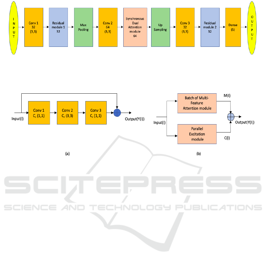
Figure 1: Proposed DNNAM Architecture model for structural component recognition. Here Conv block represents convolu-

tional operation with the ﬁrst number representing the number of ﬁlters and the next two numbers giving the ﬁlter dimension

for each channel. Dense represents the dense layer, where the ﬁrst number gives the number of nodes. The proposed syn-

chronous dual attention module is composed of a batch of multi-feature attention module and a parallel excitation module.

The number denoted in the synchronous dual attention module and residual module represents ﬁlter size.

Figure 2: (a) Proposed residual module for DNNAM architecture. Here Conv block represents convolutional operation with

the ﬁrst number representing the number of ﬁlters and the next two numbers giving the ﬁlter dimension for each channel.

(b) Proposed Synchronous dual attention module for DNNAM architecture is composed of a batch of multi-feature attention

module and a parallel excitation module.

nel attention synchronously and aggregates their re-

sults to highlight discriminative features for multiple

target structural component classes. The block dia-

gram shown in Fig. 2 (b) is comprised of two mod-

ules: a batch of multi-feature attention module and a

parallel excitation module. The batch of multi-feature

attention module (BMFA) is created to encode several

representations of extremely localised features, allow-

ing the network to pick up on even the smallest com-

ponent classes. The parallel excitation module (PEM)

is used to synchronously highlight the signiﬁcant as-

pects and lessen the impact of weak or unimportant

features as it encodes the spatial and channel informa-

tion for artefacts. To increase the impact of the syn-

chronous dual attention module, the outputs of these

two attention modules are fused together.

2.2.1 Batch of Multi-Feature Attention Module

We use a batch of multi-feature attention module

to combine several representations of the highly lo-

calised parallel feature extraction process in order to

encode relevant information from visually identical

concrete structural components. To distinguish be-

tween non-bridge, columns, beams and slabs, other

structural, and other non-structural components, this

module serves to encapsulate highly localised feature

selection mechanisms. To ensure that the most sig-

niﬁcant aspects are attended to, the attention actions

in this proposed module are repeated several times.

To produce parallel non-linear projections in feature

space, each attention module uses three dense lay-

ers to conduct synchronous computations. Here, the

input (I), is taken into account along with its corre-

sponding height, width and the number of channels.

Then, the outputs T2 and T3 are multiplied elemen-

tally, a So f tMax function is used to create the at-

tention mask, and T1 is multiplied with the attention

mask to emphasise the critical features. The identity

mapping is then carried out by the addition of an input

tensor to the output. The output of the BMFA mod-

ule, which aggregates attentive features from several

representations, is produced by adding all three of the

outputs generated by the attention operations att1, att2

and att3. Fig. 3 shows the batch of multi-feature at-

tention module.

2.2.2 Parallel Excitation Module

In order to synchronously encode salient spatial and

channel information, the convolution layer captures

local spatial features across all of the channels (He

et al., 2016; Hu et al., 2018). We must selectively

draw attention to and suppress other aspects while

Deep Neural Network Based Attention Model for Structural Component Recognition

319

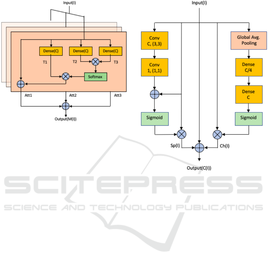
Figure 3: The Batch of multi-feature attention module is

a combination of 3 self-attention layers. In each layer, the

Input(I), together with its matching height, width, and chan-

nel count, are taken into consideration. The attention mask

is then created using the SoftMax function, the outputs T2

and T3 are multiplied elementally, and T1 is multiplied with

the attention mask to highlight the important features. After

that, the identity mapping is completed by adding an input

tensor to the output.

emphasising the channel wise discriminative struc-

tural component features. The parallel excitation

module analyses the key spatial and channel informa-

tion individually to address these issues and enhance

performance. This module includes a function that

squeezes the input tensor’s spatial plane using global

average pooling before stimulating it channel wise to

get channel information. The module can automat-

ically contain the global channel description thanks

to the channel squeezing operation, which provides

statistics for the entire image on a channel by chan-

nel basis. The following dense layers use non-linear

adaptive re-calibration to extract discriminative chan-

nels with important features while also utilising con-

textual channel information. In order to create the

channel attention feature map Ch(I) as illustrated in

Fig. 4, the output of two dense layers is activated us-

ing the sigmoid function and multiplied with the input

(I). This is carried out to emphasise the characteristics

required for channel speciﬁc identiﬁcation.

Similar to how the ﬁrst portion of the parallel exci-

tation module squeezes the channels, the second half

of the module uses convolution blocks to capture the

common spatial features present in all channels. To

avoid losing important contextual features after con-

volution, we inserted a skip connection with the input

before proceeding to the sigmoid activation function.

Figure 4: The Parallel Excitation Module examines the im-

portant Spatial, Sp(I) and Channel, Ch(I) Information Sepa-

rately. The ﬁrst half of the module uses convolution blocks

to capture the common spatial features present in all chan-

nels. The second half of the module includes a function

that squeezes the input tensor’s spatial plane using global

average pooling before stimulating it channel-wise to get

channel information.

The recovered features are spatially excited, and the

output is then multiplied by the input tensor to high-

light the crucial spatial data Sp(I). In contrast to (Woo

et al., 2018), where the spatial attention is carried out

via average and max pooling operation, the global

channel features are squeezed to extract salient spatial

information to provide spatial statistics by decreasing

the input through its channel dimension. Instead of

employing 1 × 1 convolution directly for the aggre-

gation of spatial information, another 3 × 3 convolu-

tion block is placed before it in order to aid in efﬁcient

feature extraction. Finally in this case, along with spa-

cial, Sp(I) and channel, Ch(I) information the input is

also added utilising a skip connection to prevent the

loss of crucial discriminative information and to alle-

viate the vanishing gradient problems as shown in Fig.

4. Finally, we add the outputs of the BMFA module,

M(I) and PEM module, C(I) to obtain the output of

the SDAM module as shown in Fig. 2 (b).

VISAPP 2023 - 18th International Conference on Computer Vision Theory and Applications

320

3 EXPERIMENTAL RESULTS

AND DISCUSSIONS

3.1 Bridge Component Classiﬁcation

Dataset

We have evaluated our algorithms and compared

them with the existing methods on the benchmark-

ing dataset for bridge component classiﬁcation pro-

vided by the authors (Narazaki et al., 2017; Narazaki

et al., 2020; Narazaki et al., 2018), obtained for aca-

demic research and algorithmic evaluation compari-

son purposes. This dataset includes 1,563 bridge pho-

tos in a total of 320 × 320 pixel dimensions, out of

which 1329 images are used for training and the re-

maining 234 images are used for testing. Each im-

age is classiﬁed into one of ﬁve classes: Non-bridge,

Columns (including piers), Beams and Slabs, Other

Structural (trusses, arches, cables, abutments, extraor-

dinary braces, amazing bearings, etc.), and Other

Non-structural (fences, poles, etc.).

3.2 Implementation Details

In our DNNAM model, we employ a max pooling

method that summarises the average and most acti-

vated presences of several features. To ﬁlter noisy ac-

tivations in a lower layer of a convolution network,

pooling abstracts activations in a receptive ﬁeld into

a single representative value. Spatial information

within a receptive ﬁeld is lost during pooling, even

though it aids classiﬁcation by maintaining only ro-

bust activations in upper layers. This information may

be crucial for the exact localisation needed for seman-

tic segmentation (Noh et al., 2015). We use unpooling

layers in our model, which reverse the pooling pro-

cess and reconstruct the initial size of activations, to

address this issue. This unpooling method is espe-

cially helpful for re-creating the input object’s struc-

ture.

The batch size for training methods is 16. Fol-

lowing earlier research (Narazaki et al., 2017), the

dataset has had random cropping, random ﬂipping,

and random rotation applied in addition to the cen-

tre crop. Weighted Binary cross entropy loss is used

for training. Binary cross entropy is used to compare

each of the projected probabilities to the actual class

output, which can only be either 0 or 1. The score

that penalises the probabilities based on how far they

are from the predicted value is then calculated. This

shows the degree to which the value resembles the ac-

tual. The number of classes in the dataset, in this case,

5 is used as the rank value. The setting for the learn-

ing rate, α is 0.001. In order to improve the DNNAM

Figure 5: (a) Real image, (b) ground truth image and (c)

Predicted image with more than 80% pixel accuracy. Sim-

ply put, a non-bridge component class comprised more than

80% of the original image in this situation. As a result, more

than 80% of the pixels have been accurately identiﬁed. This

example is meant to demonstrate that high pixel accuracy

does not always imply superior segmentation skills.

model, the Adam optimizer is used for optimization

strategy with β

= 0.9 and β

= 0.999. The models

are trained using the Bridge component classiﬁcation

dataset over 100 epochs. The experiments are carried

out on a system with an Intel(R) Core(TM) i7-9700

processor, 32 GB of RAM, and an NVIDIA GeForce

RTX-2080 8GB GPU card utilising the Python Keras

API and TensorFlow backend.

3.3 Performance Metrics

For comparison with the previous benchmarking

methods, we are using the following performance ma-

trices

3.3.1 Pixel Accuracy

The percentage of accurate pixel class prediction

compared to the ground truth is measured as pixel

accuracy (PA) over the test set. It is the proportion

of correctly classiﬁed pixels in our image. Now we

can take into account a situation that we encountered

throughout the project’s ﬁrst stages to reveal the prob-

lems associated with this metric. Fig. 5 (a) and (b)

show the real image and the ground truth image, re-

spectively, that was given to the model. The model is

attempting to recognise or segment structural compo-

nents in the bridge image. Fig. 5 (c) depicts the pre-

diction with more than 80% accuracy. That means,

in this case, more than 80% of the original image be-

longed to one speciﬁc class (non-bridge component

class). Therefore, more than 80% of the pixels are

identiﬁed correctly, but the remaining 20% are inac-

curate if the model assigns all pixels to that class. Be-

cause of this, even though our accuracy is great, the

model is failing to accurately predict or identify the

structural components of the image.

The example in Fig. 5 is intended to show that ex-

cellent segmentation skills are not always implied by

great pixel accuracy. When our classes are severely

Deep Neural Network Based Attention Model for Structural Component Recognition

321

out of balance, one or more classes dominate the pic-

ture while other classes make up a very minor fraction

of it. Unfortunately, this can’t be disregarded because

it can be seen in many real world data sets. As a result,

we offer substitute metrics that are more effective in

addressing this problem.

3.3.2 Mean Intersection-over-Union

One of the most used metrics in semantic seg-

mentation is the intersection-over-union (IOU), of-

ten known as the Jaccard Index. The IOU is an ex-

ceedingly effective metric that is relatively simple to

use. The IOU can be deﬁned as the area of union

between the predicted segmentation and the ground

truth divided by the area of overlap between the pre-

dicted segmentation and the ground truth. The mean

IOU (mIOU) of the picture is determined for binary

or multi-class segmentation by averaging the IOU of

each class, where IOU is given by equation 1 and is

calculated across each semantic class and then aver-

aged.

IOU =

T P

T P + FN + FP

(1)

Where T P, FN, and FP stand for true positives,

false negatives and false positives, respectively. These

terms are produced by comparing the actual labels

with those that were predicted.

Now, using the same example as pixel accuracy,

let’s try to see why this metric is superior. For sim-

plicity, let’s assume that all structural elements be-

long to the same class. Let’s compare the anticipated

segmentation to the actual or ground truths. At ﬁrst,

we determine the IOU for the structural component.

We consider the image’s overall area to be 100 pixels,

which focuses on the overlap of the structural compo-

nents ﬁrst. To check for overlapping component pix-

els, we can make the predicted segmentation on Fig. 5

on Fig. 5 (b). There are 0 overlapping structural com-

ponent pixels because the model does not identify any

pixels as structural components. The pixels from both

images that were classiﬁed as structural components

are included in the union, but not the overlapped or

intersected pixels. That is signiﬁcantly less than the

80% pixel accuracy we predicted. It is evident that it

gives a far more realistic image of how well our seg-

mentation worked, though.

3.4 Comparison with Benchmarks

The performance of the suggested architecture com-

pared to other benchmarks is summarised in Table 1.

The results from earlier techniques (Narazaki et al.,

2017; Yeum et al., 2019) are expressed in terms of

Table 1: Comparison with Pre-existing Benchmarks on the

Bridge component classiﬁcation dataset. We are consider-

ing mIOU as more important than PA, Perhaps because of

a lack of high-quality ground creation, mIOU is better than

PA on this dataset.

Benchmarking Works mIOU(%) PA(%)

CNPT - N

50.8 80.3

CPNT - Scene

- 82.4

FCN45

- 82.3

FCN45 - N

57.0 84.1

FCN45- P

56.9 84.1

FCN45- S

56.6 83.9

SegNet45- N

54.5 82.3

SegNet45 - P

55.2 82.9

SegNet45 - S

55.2 82.9

SegNet45-S - N

55.8 83.1

SegNet45-S - P

55.9 83.3

SegNet45-S - S

55.4 82.7

StructureNet

57.46 89.08

DNNAM 65.94 82.85

(Narazaki et al., 2017)

(Narazaki et al., 2020)

(Yeum

et al., 2019)

(Kaothalkar et al., 2022)

mean IOU (mIOU), and a comparison is made with

the most recent work by (Kaothalkar et al., 2022) and

(Narazaki et al., 2020), which takes into account both

mIOU and Pixel Accuracy (PA). Naive (N), Parallel

(P), and Sequential (S) models with various conﬁg-

urations are also compared in the (Narazaki et al.,

2020) paper.

The convergence curves produced during the

DNNAM network’s training are shown in Fig. 6. As

time goes on, we could see that both training and test-

ing, accuracy and mean IOU are steadily rising while

loss is decreasing. Our proposed DNNAM model

achieves a mean IOU of 65.94% with pixel wise ac-

curacy of 82.85%. Thus, when compared to all of

the previous research, our model surpasses them in

terms of mean IOU and also outperforms (Narazaki

et al., 2017; Narazaki et al., 2020; Yeum et al., 2019)

in terms of pixel wise accuracy for the prior work.

The inconsistent labelling of a few ground truths

on this dataset, also described in (Kaothalkar et al.,

2022), is a problem for performance saturation on

testing data. The average processing time of our de-

veloped model is 0.1001 seconds. Fig. 7 shows

the segmentation results of our proposed DNNAM

model on the Bridge Component Classiﬁcation test

set. To create the attention maps that help explain the

proposed network’s decision-making process, sample

images from the dataset are applied to the DNNAM

architecture are shown in Fig. 8. These attention

maps assist the network to focus on these regions au-

tomatically by emphasising higher weightage on the

VISAPP 2023 - 18th International Conference on Computer Vision Theory and Applications

322

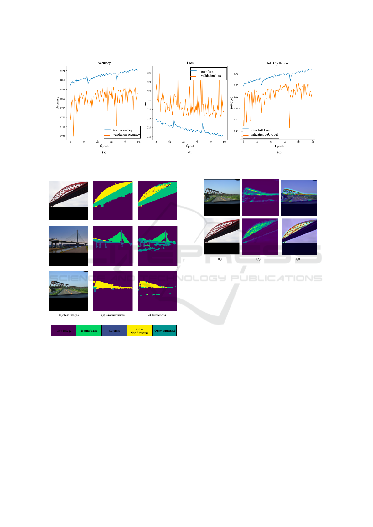
Figure 6: Performance curves generated during the training of the DNNAM network. Here blue and orange curves represent

training data and validation data accuracy over the epochs, respectively. (a) Accuracy (b) Loss and (c) IOU coefﬁcient.

Figure 7: Segmentation results of our proposed DNNAM

model. Our proposed DNNAM model yields a mean IOU

of 65.94% with pixel wise accuracy of 82.85%.

structural component regions that help to extract ro-

bust discriminatory features for their classiﬁcation.

The results are presented in terms of pixel accu-

racy on the ResNet23 model (mIOU score is taken

from (Narazaki et al., 2020)), with the naive com-

ponent classiﬁer (CPNT - N) and component clas-

siﬁer with scene information (CPNT - Scene) being

proposed in the ﬁrst benchmark on the dataset by

(Narazaki et al., 2017). The bridge component clas-

siﬁcation dataset uses the benchmark from another

study (Yeum et al., 2019). The majority of the re-

Figure 8: Attention maps obtained from the proposed

DNNAM network for sample images from the Bridge

component classiﬁcation dataset. (a) Original images are

followed by their respective (b) attention maps and (c)

heatmaps are placed side-by-side.

sults come from the various approaches reported by

(Narazaki et al., 2020), among which FCN45-N re-

ports the best mIOU of 57.0% and the best pixel

accuracy of 84.1%. If we observe the comparison

with pre-existing benchmark’s Table 1, we could see

most of Narazaki’s work yielded an average of 55%

in terms of Mean IOU values. Narazaki’s earlier

work is outperformed by recent work by (Kaothalkar

et al., 2022), which has the mIOU (57.46%) and best

pixel accuracy (89.08%) values. Mean IOU is con-

sidered the best performance metric and our proposed

DNNAM model got mIOU (65.94%). Thus our pro-

posed model DNNAM, in terms of mIOU performs

8.48% better than the previously established highest

values. Also, we could notice that all the benchmark-

ing works are generating pixel accuracy greater than

80% and our model also keeps that margin in the ex-

perimental results with 82.85% PA.

As we explained in the previous section perfor-

mance metrics, there are certain disadvantages to util-

Deep Neural Network Based Attention Model for Structural Component Recognition

323

Table 2: Assessment of DNNAM on Semantic Augmented

Make3D dataset when compared with the baseline model.

Assessment mIOU (%) PA (%)

Make3D-S (Liu et al., 2010)

Baseline ResNet-50 65.83 88.42

DNNAM 73.42 87.47

ising the performance metric pixel accuracy, hence in

our study, we are emphasising on the performance

metric mean IOU. In the early stages of our experi-

mental tests, we found that while running the model

for a few additional epochs allowed us to attain pixel

accuracy that was higher than that of the previous

works, the model was unable to correctly anticipate or

identify the structural elements of the image. Through

our analysis and studies ﬁnally, we are able to estab-

lish that when the synchronous dual attention module

and residual modules are combined as we proposed,

it can capture long-range dependencies in the feature

maps, improving the architecture’s efﬁciency and ac-

curacy.

Assessment on Semantic Augmented Make3D

Dataset: We evaluate the model’s performance

on an additional dataset, the Semantic Augmented

Make3D (Liu et al., 2010; Saxena et al., 2005; Sax-

ena et al., 2008) dataset, acquired for research and

comparison evaluation purposes. 400 training images

and 134 evaluation images from 8 separate classes

make up the Make3D-S dataset. Each image has an

input resolution of 240 × 320. This dataset is cho-

sen since it contains outdoor images of various types

of buildings and structures. The evaluation is sum-

marised in Table 2, which demonstrates that our sug-

gested DNNAM outperforms the backbone architec-

ture (ResNet-50) for the Make3D-S dataset and can be

used for the semantic segmentation task as well. Due

to the inclusion of residual module and contextual

level information encoding across spatial and chan-

nel dimensions, which provides more ﬁne-tuned fea-

ture extraction and hence improves the metric values,

results in Table 2 show superior results for the addi-

tional dataset as well.

4 ABLATION STUDIES

To demonstrate the effectiveness of the fusion of syn-

chronous dual attention modules (SDAM) and resid-

ual modules, a series of ablation study experiments

are conducted. In the ﬁrst case, the SDAM module

is eliminated and observed the results without an at-

tention mechanism. To achieve better outcomes in the

second case, we exclusively use residual modules and

vary the number of residual modules as well. The re-

sults are summarised in Tables 3 and 4. It should be

emphasised that when utilised separately, each mod-

ule does not produce the best results; only when they

are combined do they perform signiﬁcantly better at

making predictions.

4.1 Ablation Experiments on SDAM

Module

With a thorough ablation investigation, we assess

many aspects of SDAM and report the ﬁndings on

the structural component dataset (Narazaki et al.,

2017; Narazaki et al., 2020; Narazaki et al., 2018;

Kaothalkar et al., 2022). Firstly, we train the network

by retaining just residual modules, i.e., by omitting

the primary core synchronous dual attention module.

The lack of an attentive feature extraction process

in this case results in a performance drop. Due to

substantial changes and the presence of overlapped

structural components, which might have been ade-

quately distinguished by utilising the complete atten-

tion mechanism, we can notice lower performance on

the structural component dataset.

Secondly, we attempt to evaluate the signiﬁcance

of various attention processes included in the pro-

posed architecture. The parallel excitation module

(PEM) is taken out while all the remaining modules

are kept in order to investigate this. Due to the lack

of a spatial-channel attention mechanism to encode

discrete structural components, experimental results

in Table 3 show a decline in performance for recog-

nizing the structural components. The same opera-

tion is then repeated while omitting all of the batch of

multi-feature attention module (BMFA), demonstrat-

ing that the structural component dataset has lower

accuracy because it lacks the highly localised fea-

ture selection that is necessary to distinguish between

structural components that overlap and have similar

appearances.

Thirdly, while leaving the other modules in place,

we take off one of the parallel excitation module sub-

channel networks and spatial attention components at

a time to examine the effects of speciﬁc attention op-

erations on recognition performance. Table 3 shows

the structural component recognition performance by

removing one of the attention sub-networks, which

shows a reduced performance in both scenarios and

further reinforces the need for using both channel and

spatial attention components.

Finally, we double the quantity of SDAM mod-

ules to track any performance changes. Similar per-

formance is shown by the testing results, but a sin-

gle SDAM module near the core produced better re-

VISAPP 2023 - 18th International Conference on Computer Vision Theory and Applications

324

Table 3: Ablation experiments on synchronous dual atten-

tion module. This study demonstrates decreasing perfor-

mances for each of these scenarios in both performance pa-

rameters (mIOU and PA), emphasising the importance of

the proposed architecture design’s performance.

Model Description mIOU(%) PA(%)

DNNAM without

SDAM

59.59 80.10

Residual Module + Only

BMFA

63.35 81.63

Residual Module + Only

PEM

51.08 80.35

Only Spatial attention in

PEM

59.24 78.66

Only Channel attention

in PEM

58.03 79.08

BMFA with only 2 lay-

ers

61.76 81.31

BMFA with 4 layers 61.41 79.68

DNNAM with 2 SDAM 48.07 74.73

Self attention replacing

BMFA

61.06 80.61

Self attention replacing

PEM

38.55 80.23

Self attention replacing

SDAM

61.12 80.14

DNNAM 65.94 82.85

Table 4: Ablation experiments on the residual module. This

study shows decreased performances for each of these sce-

narios in performance parameters (mIOU and PA), further

highlighting the signiﬁcance of the performance of the pro-

posed architectural design.

Model Description mIOU(%) PA(%)

DNNAM without Resid-

ual Module

58.41 77.85

Only 1 Residual Module 56.86 78.41

Using 2 Residual Mod-

ule

60.08 78.59

Using 4 Residual Mod-

ule

62.30 79.52

DNNAM 65.94 82.85

sults with minimal running times. Table 3 shows

decreased performances for each of these scenarios,

further highlighting the signiﬁcance of the proposed

modules.

4.2 Ablation Experiments on Residual

Module

We conduct a broad range of experiments on the

residual module to assess the impact of various

changes and the results are summarised in Table 4.

Firstly, the proposed network is trained using only

the synchronous dual attention modules and not

any residual modules, which use fewer parameters.

However, as seen in Table 4, the classiﬁcation perfor-

mance suffers when the residual module is absent.

A deeper network results from the extraction of

local features across all channels with the assistance

of residual modules. To capture multi-scale fea-

ture representation, each residual block combines

features from all prior responses. It demonstrates

the effectiveness of a deeper network, such as a

residual module, in obtaining reliable features for the

identiﬁcation of overlapping structural components.

Moreover, these networks emphasise accurate spatial

feature estimation.

Additionally, the network can alleviate the vanish-

ing gradient problem with generalised performance

owing to the identity mappings across the residual

units. These traits of the residual module contribute to

the structural component dataset’s increased perfor-

mance. Furthermore, we tested altering the number

of residual modules in the design to see how perfor-

mance changed and discovered that keeping 3 will re-

sult in the optimal performance matrices with the least

amount of running time. We obtain decreased results

in Table 4 for each of these scenarios, further high-

lighting the signiﬁcance of the proposed modules.

5 CONCLUSION AND FUTURE

WORK

In this work, we address the challenges involved in

structural component recognition, a crucial step in the

inspection process and management of civil infras-

tructures. To improve classiﬁcation performance with

fewer parameters, our proposed DNNAM architecture

is built using synchronous dual attention modules and

residual modules, which are used to extract robust

salient discriminative features from multiple scales.

Numerous experimental results and ablation studies

on benchmarking datasets demonstrate the superiority

of the proposed DNNAM architecture as compared

to other current state-of-the-art approaches, particu-

larly in terms of the performance metric mean IOU

for multi-target and multi-class classiﬁcation prob-

lems. The classiﬁcation of additional kinds of struc-

tural components may beneﬁt from the success of the

proposed DNNAM architecture.

The structural component recognition studied in

this research is a crucial building block for au-

tonomous robot navigation in post-earthquake/natural

or other calamity disaster affected areas. The pro-

Deep Neural Network Based Attention Model for Structural Component Recognition

325

posed DNNAM system can be used in conjunction

with unmanned aerial vehicles (UAVs) to quickly

identify structural elements and can accurately detect

deterioration, anticipate how long a structure will last

and monitor large concrete structures.

REFERENCES

Bhattacharya, G., Puhan, N. B., and Mandal, B. (2021).

Stand-alone composite attention network for concrete

structural defect classiﬁcation. IEEE Transactions on

Artiﬁcial Intelligence, 3(2):265–274.

Cordonnier, J.-B., Loukas, A., and Jaggi, M. (2019). On the

relationship between self-attention and convolutional

layers. arXiv preprint arXiv:1911.03584.

Gao, Y. and Mosalam, K. M. (2018). Deep transfer learn-

ing for image-based structural damage recognition.

Computer-Aided Civil and Infrastructure Engineer-

ing, 33(9):748–768.

Guo, H., Zheng, K., Fan, X., Yu, H., and Wang, S. (2019).

Visual attention consistency under image transforms

for multi-label image classiﬁcation. In Proceedings

of the IEEE/CVF conference on computer vision and

pattern recognition, pages 729–739.

He, K., Zhang, X., Ren, S., and Sun, J. (2016). Deep resid-

ual learning for image recognition. In Proceedings of

the IEEE conference on computer vision and pattern

recognition, pages 770–778.

Hu, J., Shen, L., and Sun, G. (2018). Squeeze-and-

excitation networks. In Proceedings of the IEEE con-

ference on computer vision and pattern recognition,

pages 7132–7141.

Kaothalkar, A., Mandal, B., and Puhan, N. B. (2022). Struc-

turenet: Deep context attention learning for structural

component recognition. In Farinella, G. M., Radeva,

P., and Bouatouch, K., editors, Proceedings of the 17th

International Joint Conference on Computer Vision,

pages 567–573. SCITEPRESS.

Liang, X. (2019). Image-based post-disaster inspection of

reinforced concrete bridge systems using deep learn-

ing with bayesian optimization. Computer-Aided Civil

and Infrastructure Engineering, 34(5):415–430.

Liu, B., Gould, S., and Koller, D. (2010). Single im-

age depth estimation from predicted semantic labels.

In 2010 IEEE computer society conference on com-

puter vision and pattern recognition, pages 1253–

1260. IEEE.

Narazaki, Y., Hoskere, V., Hoang, T. A., Fujino, Y., Sakurai,

A., and Spencer Jr, B. F. (2020). Vision-based auto-

mated bridge component recognition with high-level

scene consistency. Computer-Aided Civil and Infras-

tructure Engineering, 35(5):465–482.

Narazaki, Y., Hoskere, V., Hoang, T. A., and Spencer, B. F.

(2017). Vision-based automated bridge component

recognition integrated with high-level scene under-

standing. arXiv preprint arXiv:1805.06041.

Narazaki, Y., Hoskere, V., Hoang, T. A., and Spencer Jr,

B. F. (2018). Automated vision-based bridge compo-

nent extraction using multiscale convolutional neural

networks. arXiv preprint arXiv:1805.06042.

Noh, H., Hong, S., and Han, B. (2015). Learning de-

convolution network for semantic segmentation. In

Proceedings of the IEEE international conference on

computer vision, pages 1520–1528.

Park, J., Woo, S., Lee, J.-Y., and Kweon, I. S. (2018).

Bam: Bottleneck attention module. arXiv preprint

arXiv:1807.06514.

Saxena, A., Chung, S., and Ng, A. (2005). Learning depth

from single monocular images. Advances in neural

information processing systems, 18.

Saxena, A., Sun, M., and Ng, A. Y. (2008). Make3d: Learn-

ing 3d scene structure from a single still image. IEEE

transactions on pattern analysis and machine intelli-

gence, 31(5):824–840.

Spencer, B. F., Hoskere, V., and Narazaki, Y. (2019). Ad-

vances in computer vision-based civil infrastructure

inspection and monitoring. Engineering, 5(2):199–

222.

Tan, Z., Yang, Y., Wan, J., Hang, H., Guo, G., and Li, S. Z.

(2019). Attention-based pedestrian attribute analysis.

IEEE transactions on image processing, 28(12):6126–

6140.

Vaswani, A., Shazeer, N., Parmar, N., Uszkoreit, J., Jones,

L., Gomez, A. N., Kaiser, Ł., and Polosukhin, I.

(2017). Attention is all you need. Advances in neural

information processing systems, 30.

Wang, F., Jiang, M., Qian, C., Yang, S., Li, C., Zhang, H.,

Wang, X., and Tang, X. (2017). Residual attention

network for image classiﬁcation. In Proceedings of

the IEEE conference on computer vision and pattern

recognition, pages 3156–3164.

Wang, W. and Shen, J. (2017). Deep visual attention pre-

diction. IEEE Transactions on Image Processing,

27(5):2368–2378.

Woo, S., Park, J., Lee, J.-Y., and Kweon, I. S. (2018). Cbam:

Convolutional block attention module. In Proceed-

ings of the European conference on computer vision

(ECCV), pages 3–19.

Yeum, C. M., Choi, J., and Dyke, S. J. (2019). Automated

region-of-interest localization and classiﬁcation for

vision-based visual assessment of civil infrastructure.

Structural Health Monitoring, 18(3):675–689.

Zhang, F., Chen, Y., Li, Z., Hong, Z., Liu, J., Ma, F., Han, J.,

and Ding, E. (2019). Acfnet: Attentional class feature

network for semantic segmentation. In Proceedings of

the IEEE/CVF International Conference on Computer

Vision, pages 6798–6807.

Zhou, S., Wang, J., Zhang, J., Wang, L., Huang, D., Du, S.,

and Zheng, N. (2020). Hierarchical u-shape attention

network for salient object detection. IEEE Transac-

tions on Image Processing, 29:8417–8428.

Zhu, Y., Zhao, C., Guo, H., Wang, J., Zhao, X., and Lu,

H. (2018). Attention couplenet: Fully convolutional

attention coupling network for object detection. IEEE

Transactions on Image Processing, 28(1):113–126.

VISAPP 2023 - 18th International Conference on Computer Vision Theory and Applications

326