A Study Toward Multi-Objective Multiagent Reinforcement Learning

Considering Worst Case and Fairness Among Agents

Toshihiro Matsui

Nagoya Institute of Technology, Gokiso-cho Showa-ku Nagoya Aichi 466-8555, Japan

Keywords:

Multiagent System, Multi-Objective, Reinforcement Learning, Cooperative Problem Solving, Fairness,

Leximin.

Abstract:

Multiagent reinforcement learning has been studied as a fundamental approach to empirically optimize the

policies of cooperative/competitive agents. A previous study proposed an extended class of multi-objective

reinforcement learning whose objectives correspond to individual agents, and the worst case and fairness

among the objectives was considered. However, that work concentrated on the case of joint-state-action space

that is handled by a centralized learner performing an ofﬂine learning. Toward decentralized solution methods,

we investigate the situations including on-line learning where agents individually own their learning tables

and selects optimum joint actions by cooperatively combining the decomposed tables with other agents. We

experimentally investigate the possibility and inﬂuence of the decomposed approach.

1 INTRODUCTION

Reinforcement learning (Sutton and Barto, 1998) is a

form of machine learning where an agent experimen-

tally learns its optimal policy in an environment based

on exploration and exploits with rewards/costs from

the environment. In multiagent reinforcement learn-

ing, agents cooperatively/competitively learn their

policies. As extended classes of reinforcement learn-

ing, multi-objective reinforcement learning (Liu et al.,

2015; Moffaert et al., 2013) for single agent sys-

tems and the learning for equilibrium among multiple

agents (Hu and Wellman, ; Hu et al., 2015; Awheda

and Schwartz, 2016) have been studied.

In this paper, we focus on the multi-objective rein-

forcement learning where each agent has its own ob-

jective. Improving fairness among agents is critical

in the practical domains of multiagent reinforcement

learning. For example, when cooperative robots have

limited power resources, the equalization/leveling of

resource consumption might be an issue to reduce the

inequality of robots’ lifetime.

A previous study (Matsui, 2019) proposed an ex-

tended class of multi-objective reinforcement learn-

ing whose objectives correspond to individual agents,

and the worst case and fairness among the objectives

were considered. In that study, each objective is de-

https://orcid.org/0000-0001-8557-8167

ﬁned as the total cost of actions of an agent in an

episode, and the objectives are simultaneously opti-

mized improving their fairness. For this optimization,

the multi-objective reinforcement learning has been

extended by employing a criterion that considers the

worst case and fairness, and the effect of the proposed

approach was experimentally shown in a pursuit prob-

lem domain. However, the previous work concen-

trated on the case of joint state-action space that is

handled by a centralized learner, and only a case of

off-line learning was addressed.

In related studies of multi-agent reinforcement

learning (Zhang and Lesser, 2012; Nguyen et al.,

2014), the global problem is decomposed into mul-

tiple agents. Although the agents manage their own

learning tables, they select the best joint action by per-

forming a cooperative protocol that aggregates the in-

formation of individual learning tables and optimizes

joint actions.

Toward a decentralized solution method, we ex-

tend the previous study in multi-objective reinforce-

ment learning for fairness among multiple agents to

investigate the case of learning tables decomposed to

agents with joint action selection based on the tables.

We also investigate the possibility of on-line learn-

ing with the decomposed setting. We experimentally

show the possibilities and inﬂuence of the decom-

posed approach.

Matsui, T.

A Study Toward Multi-Objective Multiagent Reinforcement Learning Considering Worst Case and Fairness Among Agents.

DOI: 10.5220/0011687100003393

In Proceedings of the 15th International Conference on Agents and Artiﬁcial Intelligence (ICAART 2023) - Volume 1, pages 269-277

ISBN: 978-989-758-623-1; ISSN: 2184-433X

 2023 by SCITEPRESS – Science and Technology Publications, Lda. Under CC license (CC BY-NC-ND 4.0)

269

2 PRELIMINARY

We present the background of our study by referring

to previous study (Matsui, 2019).

2.1 Multi-Objective Reinforcement

Learning

Reinforcement learning is a machine learning method

where an agent experientially obtains an optimal pol-

icy that is a sequence of its own actions in an environ-

ment (Sutton and Barto, 1998). An agent observes its

current state s ∈ S and performs action a ∈ A. Then

the agent receives a reward or cost value from the en-

vironment. By exploring an environment, an agent

updates its learning table that represents the values of

(s, a) ∈ S × A and selects its optimal action based on

the learning table. The learning rule of Q-learning on

minimization problems is as follows.

Q(s, a) ← (1 − α)Q(s, a) + α(c + γ min

Q(s

, a

)) .

(1)

Here Q(s, a) denotes the Q-table to be learned, and

c is the current cost received from an environment.

Parameters α and γ are the learning and discount rates,

respectively.

Multi-objective reinforcement learning has been

studied to simultaneously optimize multiple objec-

tives (Liu et al., 2015). That introduces the ap-

proaches of multi-objective optimization problems

into reinforcement learning. The above Q-leaning

with single objectives is extended to a multi-objective

Q-learning:

Q(s, a) ← (1 − α)Q

Q(s, a) + α(c

c + γ minws(v

v, Q

Q(s

, a

))) .

(2)

‘minws’ is a minimization operator based

on a weighted summation with vector v

argmin

Q(s

) for a

v · Q

Q(s

, a

). For multiple ob-

jectives, single cost values are extended to cost

vectors, and learning is performed based on the

scalarization/ﬁltering criteria of multi-objective

optimization problems. The above operation of

‘minws’ can be replaced by other operators based

on different criteria employed for multi-objective

optimization. We concentrate on the above case

of single policy learning that can be handled with

relatively reasonable computational cost.

Although a major part of studies on multi-

objective reinforcement learning addresses the case of

a single agent system with different objectives, multi-

objective optimization among individual agents can

be issues to be investigated.

2.2 Learning Joint Policy Considering

Bottleneck and Fairness

A previous study (Matsui, 2019) proposed a solu-

tion method based on multi-objective reinforcement

learning and a criterion to optimize the joint policies

of agents. Here individual agents’ total action cost

values are simultaneously optimized improving the

worst case and fairness. This approach extends multi-

objective Q-learning to employ the leximax criterion

that considers fairness and the worst case among mul-

tiple objectives. Leximax is a variant of a similar cri-

terion called leximin for maximization problems.

The leximax is deﬁned with a dictionary order on

sorted objective vectors whose values are sorted in de-

scending order (Bouveret and Lema

ıtre, 2009; Greco

and Scarcello, 2013; Matsui et al., 2018). Suppose

that v

v = [v

, ··· , v

] and v

= [v

, ··· , v

] denote the

sorted objective vectors of length K. Then order rela-

tion 

leximax

is deﬁned as: v

v 

leximax

if and only if

∃t, ∀t

< t, v

= v

∧ v

> v

. The minimization of the

objective vectors on leximax improves fairness and

the worst case cost value among the cost values. We

assume that an inherent trade-off between efﬁciency

(i.e., the total utility/cost value) and fairness is accept-

able, similar to related studies.

In this sub-section, we still use the notations

of state s and action a as those in the previous

sub-section, although the context of states/actions

changed to that of joint states/actions among agents.

We will replace these notations from Section 3. To ap-

ply leximax, the previous study adjusted the learning

and action-selection rules. For simple cases in deter-

ministic environments, the following learning rule is

applied. Here both learning rate α and discount rate γ

are set to 1.

Q(s, a) ← min

leximax

c + Q

Q(s

, a

)) , (3)

where c

c is a cost vector for current action a. The vec-

tors are compared using the leximax criterion. A ma-

jor difference from conventional methods is that cost

vector c

c for the current action is aggregated with ex-

pected future cost vectors before minimization. This

modiﬁcation aims to avoid the confusion of evalu-

ations in future actions (Section 3.2.2 of (Matsui,

2019)). For the modiﬁed learning rule, the action se-

lection is also modiﬁed to satisfy the following condi-

tion: Q

Q(s

−

, a

−

) = c

−

+ Q

Q(s, a), where Q

Q(s

−

, a

−

) is a

Q-vector for the previous state and action and Q

Q(s, a)

is a Q-vector for the current state and action. c

−

a cost vector for previous action a

−

. The actions are

ﬁltered by this condition in the current state, and the

best action is selected from the available ones. In the

initial state, the best action is selected only by refer-

ring to the learning table.

ICAART 2023 - 15th International Conference on Agents and Artiﬁcial Intelligence

270

For general cases of Equation (3) including non-

deterministic environments, the following learning

rule is applied:

Q(s, a) ← (1−α)Q

Q(s, a)+α min

leximax

c+γ Q

Q(s

, a

)) .

(4)

In this problem setting that consider the fairness

among the total cost values for individual agents’ ac-

tions in an episode, γ = 1 is preferred to evenly accu-

mulate future action cost values. The action selection

is also modiﬁed using an approximation with the lex-

imax operator for the difference between Q

Q(s

−

, a

−

)

and c

−

+ Q

Q(s, a). For current state s, it selects action

a = argmin

leximax

((c

−

+ Q

Q(s, a

)) −Q

Q(s

−

, a

−

)) .

(5)

Ties are broken with

a = argmin

leximax

−

+ Q

Q(s, a

)). (6)

In the previous study (Matsui, 2019), several ex-

perimental investigations were performed in a simple

case where the learning and action phases were sep-

arated. In a learning phase, every joint state-action

pair is repeatedly scanned to propagate the informa-

tion in the learning tables. In an action phase, from

the initial states of the agents, a sequence of the best

actions is selected based on the learning results and

the immediate cost vectors of the current actions un-

til agents reach a goal state. Since the previous study

only addressed the case of joint state-action space that

is learned with a single learning table, therefore, ad-

ditional investigations are necessary toward an exten-

sion to cooperative learning by multiple agents.

2.3 Multiagent Reinforcement Learning

with Cooperative Joint Action

Selection

In general multiagent reinforcement learning, each

agent has its own learning table and cooperatively/-

competitively performs learning. A top-down ap-

proach in multiagent cases is the decomposition and

approximation of a single learning table for joint ac-

tions. In such methods, agents individually learn with

their own tables but cooperatively determine their best

joint actions by solving an optimization problem that

is built by combining the information in decomposed

tables. In related studies (Zhang and Lesser, 2012;

Nguyen et al., 2014), agents cooperatively determine

their best joint action by solving a Distributed Con-

straint Optimization Problem (DCOP) (Fioretto et al.,

2018), which is a class of general combinational opti-

mization problems in decentralized settings.

Hunter

Target

Figure 1: Pursuit problem domain (Matsui, 2019).

As an extended class of DCOPs, the asymmet-

ric multi-objective DCOP has been proposed (Matsui

et al., 2018; Matsui, 2022). In this problem, objec-

tive functions between pairs of agents are asymmet-

rically deﬁned to represent the individual evaluations

of agents. These individual objective functions are

aggregated into the objective values of agents, and

then this multi-objective problem is solved by a de-

centralized solution method using leximin for the op-

timization criterion. As shown in Section 2.2, a pre-

vious multi-objective reinforcement learning (Matsui,

2019) method optimized the joint policies based on

leximax, which is a variant of leximin for minimiza-

tion problems. Therefore, there are opportunities to

decompose this learning process to individual agents

with joint action selection by the leximin (leximax)

based decentralized optimization method. Several

fundamental investigations are necessary on the inﬂu-

ences of the decomposition.

2.4 Pursuit Problem Domain

We employ an example domain of the pursuit prob-

lem presented in a previous study (Matsui, 2019). As

shown in Fig. 1, hunter agents pursuit a target agent

in a torus grid world. An agent can move to one of

the cells adjoining its current location. The two ac-

tions of hunters are to move closer to the targets or

to remain in their current locations. Such simpliﬁca-

tion conserves the action space, and the directions of

the hunter agent moves are deterministically selected

with a ﬁxed tie-break rule. The target moves to max-

imize the minimum distance to the hunters. Depend-

ing on the settings, one of the multiple best actions by

the target is deterministically or non-deterministically

selected. From their initial locations, the agents iter-

ate the observation of states and the selection of ac-

tions. An episode terminates when one hunter and the

target are in the same cell. To eliminate noise, the

observations of agents are complete. Each hunter re-

ceives its individual cost value 1 or 0 for a move or

a stay. In addition, a sufﬁciently large cost value is

given to all the hunters when all of them stay at their

current location. Without this rule or similar knowl-

A Study Toward Multi-Objective Multiagent Reinforcement Learning Considering Worst Case and Fairness Among Agents

271

edge/signals, all hunters in this problem domain will

simply learn an inappropriate joint action where they

select no move to reduce action costs. The goal of

the problem is to learn the joint policy that reduces

the cost values of hunter agents and improves fairness

and the worst case as possible. In the previous study,

the learning method that employs a single learning ta-

ble containing objective vectors of hunters was per-

formed on a joint-action space for the entire system.

We basically inherit this example problem domain

to analyze our methods. In addition, as mentioned

below, we modiﬁed the handling of inhibited joint ac-

tions where no agent moves so that such cases are ex-

cluded from action spaces by an action shaping.

3 LEARNING FAIR POLICIES IN

DECOMPOSED SETTINGS

Toward decentralized solution methods extending the

previous study (Matsui, 2019), we investigate the sit-

uations where each agent owns its learning table and

selects optimum joint actions by combining the de-

composed tables.

3.1 Decomposition of Problems

We decompose the single learning table of joint state-

action spaces Q

Q(s

s, a

a) to multiple tables Q

s, a

) for

pairs of joint state space and individual action space

of agent i. Here s

s ∈ S

S and a

a ∈

∏

A explicitly de-

note joint states and joint actions, and A denotes a

common set of each agent’s actions. We still em-

ploy joint states s

s of all agent locations including the

target agent for complete observation. By this mod-

iﬁcation, the size of learning table is reduced from

S| × |A|

|H|

to |H| × |S

S| × |A|, where |H| denotes the

number of hunter agents. Therefore, each agent only

learns the cost values of its own actions. However,

each agent should cooperate with the others to deter-

mine joint actions by a protocol. We focus on this ap-

proximated situation in multi-objective problems with

leximax criterion. In addition, to simplify the learning

process, we remove a large cost value of a joint action

for which all the hunter agents stop and introduce an

action shaping that inhibits all-stop joint action. In

cooperative situations, such an action shaping can be

applied within the decision-making process of joint

actions among agents.

1 (Initialize agents location. Globally synchronized time step

t ← 0.)

2 Initialize its own learning table Q

s, a

3 Until goal state do begin

4 Observe current joint state s

including its current.

5 Find the best joint action

for s

by cooperatively solving

a multi-objective optimization problem based on

learning tables of all the agents.

6 Perform an action referring its own action ˆa

i,t

in the best

joint action

7 Observe new joint state s

t+1

and receive cost c

8 Find the best joint action

t+1

for the new joint state s

t+1

by cooperatively solving a multi-objective

optimization problem based on learning tables of all

the agents..

9 Update Q

, ˆa

i,t

) using Q

, ˆa

i,t

), Q

t+1

, ˆa

i,t+1

) and

cost c

10 (t ← t +1.)

11 end.

Figure 2: Learning with decomposed learning table and co-

operative problem solving to determine joint action (agent

i).

3.2 Cooperation of Agents by

Optimization of Joint Actions

We assume an approach that resembles previous

work (Zhang and Lesser, 2012; Nguyen et al., 2014)

where agents individually learn with their own tables

but cooperatively determine their best joint actions.

The cooperation problem is translated to a DCOP that

is also commonly represented by a constraint graph,

and the problem is solved using a solution method.

In our case, the relationship among agents is simply

represented as a fully connected constraint graph with

unary function nodes of Q

. While the previous stud-

ies addressed single objective problems with the tra-

ditional summation criterion of cost/utility values, we

address a similar approach to multi-objective prob-

lems with a leximax criterion. Although several solu-

tion methods that aggregate individual objective val-

ues with leximin/leximax criterion are available (Mat-

sui et al., 2018; Matsui, 2022), we emulate an exact

solution method in a simulator to simply implement

the ﬁrst analysis.

The total ﬂow of the learning, including coopera-

tive problem solving for the determination of joint ac-

tions, is shown in Fig. 2. After the initialization (lines

1-2), the agents repeat both their learning and action

processes (lines 3-11). In each iteration, agents ﬁrst

observe their current joint state s

including the lo-

cations of all the hunter agents and the target agent

(line 4). Then the agents determine their joint action

in s

(line 5). To compute their best joint action,

agents cooperate to aggregate the information of their

tables and to solve a selection problem for joint ac-

tions. Here the agents solve the following problem

based on Equation (5) in most cases.

ICAART 2023 - 15th International Conference on Agents and Artiﬁcial Intelligence

272

= argmin

leximax

a∈

∏

⊕

(

i,t−1

+ Q

, a

↓a

)) − Q

t−1

, a

i,t−1

))) ,

(7)

where ⊕ is the constructor operator of sorted ob-

jective vectors. a

i,t−1

is the action in the previous

state, and c

i,t−1

is the cost value received in the previ-

ous state. a

↓a

denotes a projection from joint action

a to an action of agent i. In the initial state, terms of

the previous state are ignored. The problem for other

cases shown in Equation (6) is similarly decomposed

and aggregated. Then each agent i performs an action

i,t

, considering its own part ˆa

i,t

of the selected joint

action

(line 6), observes new joint state s

t+1

, and

receives its own cost c

i,t

(i.e., negative reward) from

the environment (line 7).

Each agent performs learning with the received

cost value and its own learning table, Since Q-

learning calculates the minimum expected cost value

(vector) for future actions, agents also cooperatively

solve the selection problem of the best joint action

t+1

in new state s

t+1

(line 8). Here the agents solve

the following problem that is a part of Equation (4).

t+1

= argmin

leximax

a∈

∏

⊕

i,t

+ γQ

t+1

, a

↓a

)) (8)

With its own part ˆa

i,t+1

of the selected joint action

t+1

, each agent calculates its related cost values and

updates its own learning table (line 9):

, a

i,t

) ←

(1 − α) Q

, a

i,t

) + α (c

i,t

+ γ Q

t+1

, ˆa

i,t+1

)) .

(9)

In the ﬁrst part of our experiment, we separately

perform the learning and action phases by decom-

posing the above on-line learning to sufﬁciently and

evenly scan the state-action space like Bellman-Ford

algorithm instead of Monte Caro method.

3.3 Experimental Analysis Of On-Line

Learning

In the analysis presented in the previous study (Mat-

sui, 2019), a learning phase was separated from an

action phase so that the learning process sufﬁciently

covers the joint state-action space. We also investigate

the case of on-line learning used in general reinforce-

ment learning.

There are several issues related to the behaviors

of agents that perform the learning in an explore-

and-exploit manner. One is that agents should im-

prove fairness and the worst case among their poli-

cies. Therefore, the discount rate of the reinforcement

learning should ideally be 1 to evenly evaluate the cost

of each action. Agents will be highly affected by the

estimated future costs that contain large errors in the

earlier steps of exploration.

In addition, convergence issues emerge due to

aliasing by decomposed learning tables. We exper-

imentally investigate the inﬂuence of the settings in

this class of problems.

4 EVALUATION

4.1 Settings

We experimentally evaluated our proposed approach

on the pursuit problem domain shown in Section 2.4

with deterministic and non-deterministic settings.

While the deterministic target agent selects one of its

best moving directions with a ﬁxed order on the direc-

tions, the non-deterministic target agent randomly se-

lects one of their best moving directions with uniform

distribution. The non-deterministic tie-break on the

best moves causes a small noise and affects the learn-

ing process. All hunter agents always select one of

their best moving directions with a ﬁxed order on the

directions. We set the cutoff iteration of agent moves

in an episode to 500.

We performed two cases of experiments. In the

ﬁrst, the learning and action selection phases were

separated, similar to the previous study, to learn by

evenly scanning the state-action space like Bellman-

Ford algorithm. In the second experiment, the agents

performed on-line learning by exploring their en-

vironment. Due to the limitation of memory us-

age and computational time to handle multiple and

multi-objective Q-tables with complete observation of

states, we addressed the size of problems up to 5 × 5

and 7 × 7 grids for the off-line and on-line settings.

We employed initial value α

of learning rate α

with decay coefﬁcient α

multiplied to α at each

episode. Also, we typically employed discount pa-

rameter γ = 1 to accumulate the future action cost

values evenly. In the second case of experiment, we

employed ε-greedy method, and its parameters were

initial value ε

of random-walk probability ε and de-

cay coefﬁcient ε

multiplied to ε at each episode.

We compared two cases of scalarization/ﬁltering

criteria of summation (sum) and leximax (lxm). In the

case of ‘sum’, the rule in Equation (2) was decom-

posed for the multiple learning tables in the agents

like in the case of lxm. Here weight vector v

v of the

summation was an all-one vector. Namely, it was de-

ﬁned as almost equivalent to the traditional summa-

tion of cost values. However, the decomposition of

the summation case is also different from the previ-

ous study that has single tables of joint state-action

A Study Toward Multi-Objective Multiagent Reinforcement Learning Considering Worst Case and Fairness Among Agents

273

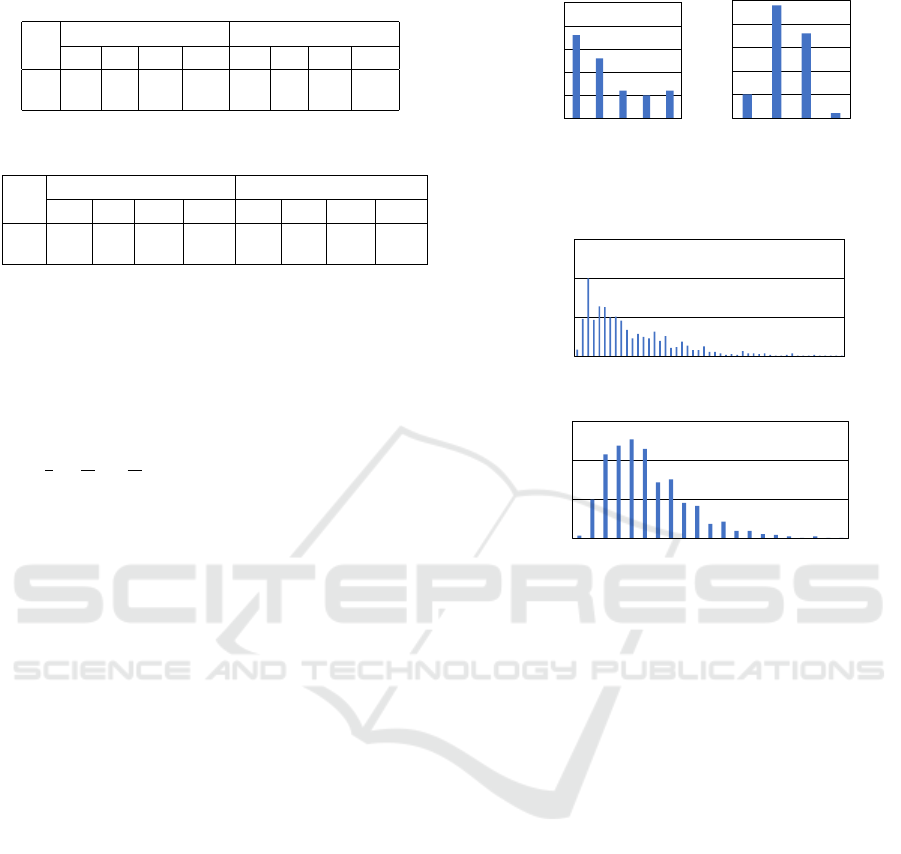
Table 1: Moving cost (deterministic, α

= 0.5, α

= 0.95,

averaged for trials).

alg. 4 × 4 grid 5 × 5 grid

min. ave. max. Theil min. ave. max. Theil

sum 0.1 1.5 3.9 0.666 0.8 2.6 4.9 0.247

lxm 0.6 1.3 2.1 0.180 1.5 2.6 4.4 0.113

Table 2: Moving cost (non-deterministic, α

= 0.5, α

0.95, averaged for trials).

alg. 4 × 4 grid 5 × 5 grid

min. ave. max. Theil min. ave. max. Theil

sum 0.9 3.7 7.8 0.354 4.1 10.1 16.7 0.157

lxm 1.5 2.7 3.9 0.109 3.5 5.3 7.1 0.064

spaces, and will be affected by the decomposition.

Since the value of leximax cannot be directly rep-

resented, we evaluated the results by the average,

minimum, and maximum cost values of the agents’

moves during the episodes. In addition, the Theil

index that is a measurement of inequality is evalu-

ated. For n objectives, Theil index T is deﬁned as

T =

∑

¯v

log

¯v

, where v

is the utility or the cost

value of an objective, and ¯v is the mean utility value

for all the objectives. When all the objective values

are identical, the Theil index takes minimum value 0.

Due to our problem setting, the Theil index is evalu-

ated for the agents’ moving costs although it is origi-

nally deﬁned for incomes.

4.2 Results: Separated Learning and

Action Selection Phases

We ﬁrst show the results of experiment where the

learning and action selection phases are separated. In

the learning phase, we scanned the whole joint state-

action space 100 times. We set learning rate α by pre-

liminary experiments, and discount rate γ was set to

1. In the action selection phase after learning, we set

the initial locations of the hunter agents to four cor-

ner cells of a grid world and varied the target’s initial

location except for the goal situations. Note that the

environment was actually a torus world. The results

were averaged for all the initial locations of the target.

In all the experiments with these settings, the agents

completed the episodes within the cut-off iteration of

their moves.

Table 1 shows the learning results of moving cost

in the deterministic cases. Ideally, ‘sum’ should re-

duce the average cost values among the agents, and

lxm should reduce the maximum cost values if there

is no noise. In the actual results, the maximum cost

value and the Theil index value were relatively small

for lxm. On the other hand, there were cases where

0 1 2 3 5

Count

Move cost

Sum

0 1 2 3

Count

Move cost

Lxm

Figure 3: Histogram of moving cost (deterministic, 5 × 5

grid, α

= 0.5, α

= 0.95, for all trials).

100

150

0 3 6 9 12151821242730333639435579

Count

Move cost

Sum

100

150

0 2 4 6 8 10 12 14 16 19 22

Count

Move cost

Lxm

Figure 4: Histogram of moving cost (non-deterministic, 5×

5 grid, α

= 0.5, α

= 0.95, for all trials).

the average cost value for lxm was also smaller than

that for sum. We found relatively large perturbation in

the learning process and the results even in the deter-

ministic cases. A possible reason is the aliasing sim-

ilar to partial observation due to the decomposition

of the global learning table into those of individual

agents. Our result revealed the necessity of further

studies to improve convergence, although the decay

coefﬁcient to learning rate mitigated the issue.

Table 2 shows the learning results of moving cost

in the non-deterministic cases. While there were

some inﬂuence of noise in the target’s actions, the

maximum cost value and the Theil index value were

relatively small for lxm. Figures 3 and 4 show the

histograms of the moving-cost values of the agents

in the experiment. Here the result were accumu-

lated for all the episodes without averaging for each

episode. For lxm in the deterministic settings, agents

moved relatively fairly and the range of the moving-

cost values was rather narrow. The results of the non-

deterministic settings were similar, while there were

several outliers of the maximum moving-cost values

due to noise.

ICAART 2023 - 15th International Conference on Agents and Artiﬁcial Intelligence

274

0.05

0.1

0.15

0.2

0.25

1.E+04

1.E+05

2.E+05

3.E+05

4.E+05

5.E+05

6.E+05

7.E+05

8.E+05

9.E+05

1.E+06

Theil

Cost

Episode

min ave

max Theil

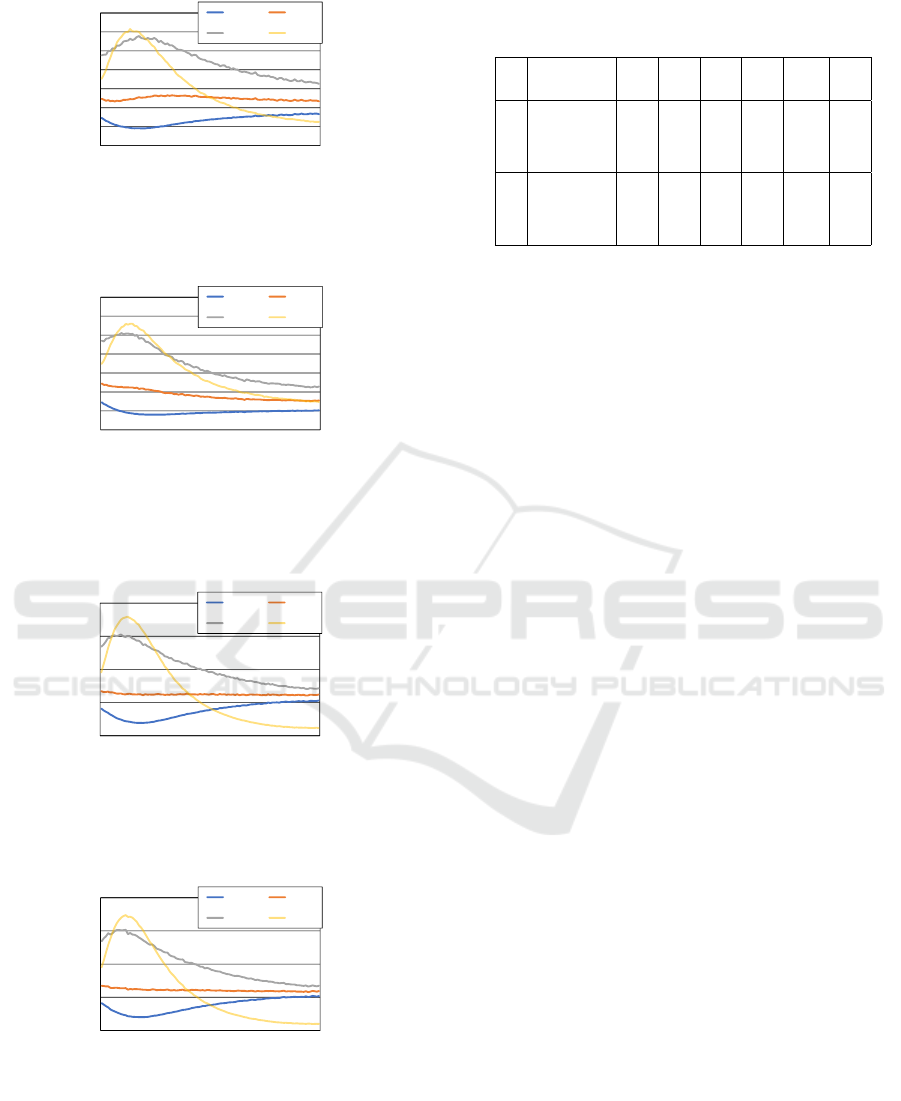
Figure 5: Learning curve (deterministic, 7 × 7 grid, α

0.5, α

= 0.999995, γ = 1, ε

= 0.5, ε

= 0.99999, sum).

0.05

0.1

0.15

0.2

0.25

1.E+04

1.E+05

2.E+05

3.E+05

4.E+05

5.E+05

6.E+05

7.E+05

8.E+05

9.E+05

1.E+06

Theil

Cost

Episode

min ave

max Theil

Figure 6: Learning curve (deterministic, 7 × 7 grid, α

0.5, α

= 0.999995, γ = 1, ε

= 0.5, ε

= 0.99999, lxm).

0.05

0.1

0.15

0.2

0.25

0.3

100

150

200

1.E+04

1.E+05

2.E+05

3.E+05

4.E+05

5.E+05

6.E+05

7.E+05

8.E+05

9.E+05

1.E+06

Theil

Cost

Episode

min ave

max Theil

Figure 7: Learning curve (non-deterministic, 7 × 7 grid,

= 0.5, α

= 0.999995, γ = 1, ε

= 0.5, ε

= 0.99999,

sum).

0.05

0.1

0.15

0.2

0.25

0.3

100

150

200

1.E+04

1.E+05

2.E+05

3.E+05

4.E+05

5.E+05

6.E+05

7.E+05

8.E+05

9.E+05

1.E+06

Theil

Cost

Episode

min ave

max Theil

Figure 8: Learning curve (non-deterministic, 7 × 7 grid,

= 0.5, α

= 0.999995, γ = 1, ε

= 0.5, ε

= 0.99999,

lxm).

4.3 Results: On-Line Learning

We next show the results of experiment when the

agents performed on-line learning. In this experi-

Table 3: Moving cost averaged for every 100 episodes in

last steps (non-deterministic, non-deterministic, 7 × 7 grid,

= 0.5, α

= 0.999995, γ = 1, ε

= 0.5, ε

= 0.99999).

alg 100 episodes 9996 9997 9998 9999 10000 ave.

to (×10

)

sum min. 56.6 50.2 53.2 49.9 49.7 51.9

ave. 66.7 58.8 61.5 59.2 58.6 61.0

max. 76.6 67.7 70.5 68.1 68.6 70.3

Theil 0.015 0.026 0.017 0.016 0.020 0.019

lxm min. 47.6 50.8 52.5 58.9 46.9 51.4

ave. 55.2 57.7 60.0 66.9 54.0 58.8

max. 63.3 65.3 67.9 75.6 61.2 66.6

Theil 0.017 0.014 0.023 0.014 0.017 0.017

ment, we set the initial locations of the hunter agents

to four corner cells of a 7 × 7 grid world (actually a

torus world) and varied the target’s initial location ex-

cept for the goal situations. With extensive prelimi-

nary experiments, we selected initial learning rate α

learning decay coefﬁcient α

, discount rate γ, initial

random-walk probability ε

and decay coefﬁcient ε

of ε-greedy method. The cut-off iteration of agents’

moves in an episode was set to 500, and we performed

the experiments until 10

episodes.

Figures 5 and 6 show the learning curves of the

cost values in the case of the deterministic settings.

The results plotted in the graphs are average values

for every 1000 episodes. We found that the average

cost values slightly changed from those in the initial

state, while the maximum cost values and the Theil

index values relatively decreased. There were rela-

tively large perturbation in the learning process due

to the decomposed learning tables and the agents’ ex-

ploration. However, in the case of lxm with discount

rate γ = 1 shown in Fig. 6, the maximum (and av-

erage) cost values were relatively smaller than those

of ‘sum’ shown in Fig. 5. In addition, we observed

that the cost values for lxm with γ = 1 were relatively

small in comparison to the cases of γ = 0.5 and 0.75.

It reveals that the correct scale of the estimated future

cost values is important for this problem domain.

Figures 7 and 8 show the learning curves of cost

values in the case of non-deterministic settings. Due

to noise in the problem settings and the exploration,

the results of both methods were similar. However,

for lxm, the maximum cost value and the Theil in-

dex value were slightly smaller than those of ‘sum’

in average among last episodes of the experiment as

shown in Table 3. Here we show average values for

every 100 episodes to emphasize perturbations.

5 DISCUSSION

Our major contribution is the investigation on the pos-

sibility of decomposed learning process including on-

A Study Toward Multi-Objective Multiagent Reinforcement Learning Considering Worst Case and Fairness Among Agents

275

line learning based on the previous approach (Matsui,

2019). For our ﬁrst investigation, we concentrated on

a case where agents have complete observation of an

environment like in the previous study. On the other

hand, the decomposition of learning tables caused the

aliasing similar to partial observation that affected the

learning process. As a result, a relatively large per-

turbation was caused in the learning process. Since

the solutions of the investigated class of problems re-

quire relatively accurate expected future cost values,

the noise due to the aliasing should be avoided as

much as possible. Mitigation of the inﬂuence of the

aliasing and analysis of the allowable range of noise

are a directions of future studies.

To improve the stability of the learning process,

several approaches, including dynamic tuning of the

learning parameters, extending the exploration strate-

gies and ﬁltering the policies, might be effective.

Since the conventional simple aggregation of esti-

mated future cost values mixes different policies,

some analysis of the inﬂuence of such an aggrega-

tion is required to improve the learning rules. More-

over, there might be appropriate exploration strategies

to optimize fairness among the agents’ policies.

While we investigated a case of decomposed

learning tables aiming the class of multiagent rein-

forcement learning where agents select their joint ac-

tion by cooperatively solving an optimization prob-

lem, there are different cooperation approaches in-

cluding reward shaping techniques (Agogino and

Tumer, 2004; Devlin et al., 2014). How such tech-

niques including game theoretic approaches can be

applied to our investigated problem will be an inter-

esting issue.

6 CONCLUSION

We investigated the decomposition of multi-objective

reinforcement learning that considers fairness and the

worst case among agents’ action costs toward decen-

tralized multiagent reinforcement learning. Our ex-

perimental results identiﬁed the possibility of our pro-

posed approach and revealed the inﬂuence of decom-

posed learning tables on the stability of learning. Our

future work will include a detailed and theoretical

analysis of the learning process and improving our

proposed method for more stable learning with dis-

tributed protocols among agents.

ACKNOWLEDGEMENTS

This work was supported in part by JSPS KAKENHI

Grant Number JP22H03647.

REFERENCES

Agogino, A. K. and Tumer, K. (2004). Unifying tempo-

ral and structural credit assignment problems. In the

Third International Joint Conference on Autonomous

Agents and Multiagent Systems, volume 2, pages 980–

987.

Awheda, M. D. and Schwartz, H. M. (2016). Exponen-

tial moving average based multiagent reinforcement

learning algorithms. Artiﬁcial Intelligence Review,

45(3):299–332.

Bouveret, S. and Lema

ıtre, M. (2009). Computing leximin-

optimal solutions in constraint networks. Artiﬁcial In-

telligence, 173(2):343–364.

Devlin, S., Yliniemi, L., Kudenko, D., and Tumer, K.

(2014). Potential-based difference rewards for mul-

tiagent reinforcement learning. In the 13th Interna-

tional Conference on Autonomous Agents and Multia-

gent System, pages 165–172.

Fioretto, F., Pontelli, E., and Yeoh, W. (2018). Distributed

constraint optimization problems and applications: A

survey. Journal of Artiﬁcial Intelligence Research,

61:623–698.

Greco, G. and Scarcello, F. (2013). Constraint satisfac-

tion and fair multi-objective optimization problems:

Foundations, complexity, and islands of tractability.

In Proc. 23th International Joint Conference on Arti-

ﬁcial Intelligence, pages 545–551.

Hu, J. and Wellman, M. P. Nash Q-learning for General-

sum Stochastic Games. Journal of Machine Learning

Research.

Hu, Y., Gao, Y., and An, B. (2015). Multiagent reinforce-

ment learning with unshared value functions. IEEE

Transactions on Cybernetics, 45(4):647–662.

Liu, C., Xu, X., and Hu, D. (2015). Multiobjective rein-

forcement learning: A comprehensive overview. IEEE

Transactions on Systems, Man, and Cybernetics: Sys-

tems, 45(3):385–398.

Matsui, T. (2019). A Study of Joint Policies Considering

Bottlenecks and Fairness. In Proc. 11th International

Conference on Agents and Artiﬁcial Intelligence, vol-

ume 1, pages 80–90.

Matsui, T. (2022). Study on Applying Decentralized Evo-

lutionary Algorithm to Asymmetric Multi-objective

DCOPs with Fairness and Worst Case. In Proc. 14th

International Conference on Agents and Artiﬁcial In-

telligence, volume 1, pages 417–424.

Matsui, T., Matsuo, H., Silaghi, M., Hirayama, K., and

Yokoo, M. (2018). Leximin asymmetric multiple

objective distributed constraint optimization problem.

Computational Intelligence, 34(1):49–84.

Moffaert, K. V., Drugan, M. M., and Now

e, A. (2013).

Scalarized multi-objective reinforcement learning:

ICAART 2023 - 15th International Conference on Agents and Artiﬁcial Intelligence

276

Novel design techniques. In 2013 IEEE Symposium on

Adaptive Dynamic Programming and Reinforcement

Learning, pages 191–199.

Nguyen, D. T., Yeoh, W., Lau, H. C., Zilberstein, S., and

Zhang, C. (2014). Decentralized multi-agent rein-

forcement learning in average-reward dynamic dcops.

In Proc. 28th AAAI Conference on Artiﬁcial Intelli-

gence, pages 1447–1455.

Sutton, R. S. and Barto, A. G. (1998). Reinforcement learn-

ing : an introduction. MIT Press.

Zhang, C. and Lesser, V. (2012). Coordinated multi-agent

learning for decentralized pomdps. In Proc. 7th An-

nual Workshop on Multiagent Sequential Decision

Making Under Uncertainty held in conjunction with

AAMAS.

A Study Toward Multi-Objective Multiagent Reinforcement Learning Considering Worst Case and Fairness Among Agents

277