On Attribute Aware Open-Set Face Veriﬁcation

Arun Kumar Subramanian

and Anoop Namboodiri

Center for Visual Information Technology, International Institute of Information Technology, Hyderabad, India

Keywords:

Open-Set Face Veriﬁcation, Deep Face Embedding, Template Matching, Facial-Attribute Covariates, Deep

Neural Networks, Transfer Learning.

Abstract:

Deep Learning on face recognition problems has shown extremely high accuracy owing to their ability in

ﬁnding strongly discriminating features. However, face images in the wild show variations in pose, lighting,

expressions, and the presence of facial attributes (for example eyeglasses). We ask, why then are these vari-

ations not detected and used during the matching process? We demonstrate that this is indeed possible while

restricting ourselves to facial attribute variation, to prove the case in point. We show two ways of doing so. a)

By using the face attribute labels as a form of prior, we bin the matching template pairs into three bins depend-

ing on whether each template of the matching pair possesses a given facial attribute or not. By operating on

each bin and averaging the result, we better the EER of SOTA by over 1 % over a large set of matching pairs.

b) We use the attribute labels and correlate them with each neuron of an embedding generated by a SOTA

architecture pre-trained DNN on a large Face dataset and ﬁne-tuned on face-attribute labels. We then suppress

a set of maximally correlating neurons and perform matching after doing so. We demonstrate this improves

the EER by over 2 %.

1 INTRODUCTION

Face images when trained on large-scale public

databases, such as Vggface2 has the ability to cre-

ate embedding that is capable of ensuring veriﬁca-

tion accuracy of over 99.5 on some public evalua-

tion datasets. However, when these trained mod-

els are inferenced on various test-datasets unseen

during train (open-set veriﬁcation) the resulting em-

bedding are known to capture variations such as

soft-biometrics and facial attributes. For exam-

ple, (Terh

orst et al., 2020a) shows that attribute-rich

dataset such as CelebA (open-set veriﬁcation), the

resulting embeddings are capable of capturing soft-

biometrics such as age, demographics, ethnicity, and

facial-hair. Also, (O’Toole et al., 2018) that attributes

clustered images are found at different layers of the

face-space. Also, (Sankaran et al., 2021) have shown

that templates constructed for similar poses yielded

better veriﬁcation accuracy. Finally, we too experi-

mented and observe as shown in Fig1 that the pres-

ence or absence of an attribute in probe and gallery in-

ﬂuences the veriﬁcation accuracy of the attribute com-

puted from the same embedding. This ﬁnding of ours

https://orcid.org/0000-0003-1123-1720

https://orcid.org/0000-0002-4638-0833

on the speciﬁed facial attribute, motivated us to devise

methods for better veriﬁcation/matching by exploit-

ing the prior knowledge of the presence or absence of

a speciﬁc facial attribute. This prior knowledge can

be obtained by a trained attribute detector or human-

labels if available. For demonstrating our idea in this

paper, we use human-labels available in the datasets

we are testing in. The two proposed methods to obtain

better veriﬁcation performance exploiting the prior in-

formation are discussed in the next two sub-sections.

While the third subsection discusses the need and rel-

evance of having two such methods.

1.1 Conﬁguration Speciﬁc Operating

Threshold

In the ﬁrst method, henceforth referred to as, CSOT

(Conﬁguration Speciﬁc Operating Threshold) we cre-

ate three bins consisting of matching template pairs

where both the templates of the matching pair in the

ﬁrst bin, possess the attribute, and in the second bin

one template does and other does not, and in the

third bin, both do not possess facial attribute, and use

different matching thresholds for each of these bins.

We refer to these three bins/conﬁgurations/protocols

henceforth as att-att (short for attribute-attribute), att-

Subramanian, A. and Namboodiri, A.

On Attribute Aware Open-Set Face Veriﬁcation.

DOI: 10.5220/0011687000003417

In Proceedings of the 18th International Joint Conference on Computer Vision, Imaging and Computer Graphics Theory and Applications (VISIGRAPP 2023) - Volume 5: VISAPP, pages

161-172

ISBN: 978-989-758-634-7; ISSN: 2184-4321

 2023 by SCITEPRESS – Science and Technology Publications, Lda. Under CC license (CC BY-NC-ND 4.0)

161

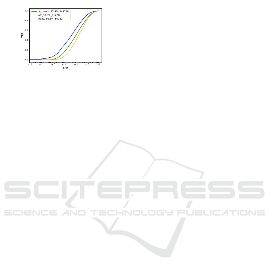
Figure 1: A plot for the ’Smiling’ attribute, showing that

matching operates differently depending on whether probe

and gallery have the attribute in question or not. att in the

plot above refers to probe and gallery having attribute. att-

noatt is probe having the attribute and gallery without the

attribute. noatt refers to probe and gallery not having the

attribute.

noatt (short for attribute-no attribute) and noatt-noatt,

our work leverages the facial attribute labels on chal-

lenging IJB-C dataset to create the three bins, each

consisting of probe and gallery samples, conditioned

on the bin type i.e att-att/att-noatt/noatt-noatt. We

have created an extensive set of 60000 pairs for each

bin, and ran an inference of SOTA networks on the

same to determine the threshold

1.2 Attribute Aware Face Embedding

and Suppression

In the second method, hence referred to as,

AAFES(Attribute Aware Face Embedding and Sup-

pression) given the understanding that veriﬁcation ac-

curacy is inﬂuenced by the presence of an attribute,

we create an attribute-aware embedding and then de-

vised a method to isolate the neurons most sensitive to

a given facial-attribute, and suppress it. The concep-

tion of this embedding is that it should leverage the

learning from a pre-trained state-of-the-art network

on a large data and to this effect we for pre-trained

InceptionResnetV1 trained on VGGFace, and thus

serve as a face-embedding, while we ﬁne-tune the

later layers of the DNN to serve as attribute classiﬁer,

hence making it more plausible to suppress the neu-

rons. We had to train such as attribute-aware face em-

bedding because existing attribute embeddings aren’t

suited for face veriﬁcation. For instance, while there

have been efforts to learn the correlations between la-

bels of CelebA data, and effort was made to take the

low/mid-level representation in (Chen et al., 2021), it

is still based on the limited data of CelebA which is

high class imbalanced and hence doesn’t suit our goal

of having high identity learning in addition to the at-

tributes. Even this work (Chen et al., 2021) wonders

in the conclusion section if pre-training could have

helped learn a more robust attribute classiﬁer.

We noticed, with a drop of about 5 percent face

veriﬁcation accuracy after the training above, the at-

tribute recognition accuracy remains intact at 93,99.6

and 96 percent for attributes Smiling, Eyeglasses, and

Mustache respectively. The veriﬁcation accuracy was

assessed using probe/gallery template match detailed

in section 4, while the attribute recognition accuracy

was measured from the fully connected network out-

put.

1.3 Need for the Two Approaches

In this section, we discuss the need and application

areas for two approaches stated above i.e. 1.1 and

1.2.

The CSOT approach is relevant when we would

like to directly use SOTA face veriﬁcation models

(both public and COTS), with no access or resources

to train our own. We can directly inference the above

models over a pool of attribute-labelled dataset, and

determine the operating threshold for att-att, att-noatt,

noatt-noatt conﬁgurations.

The AAFES approach is primarily relevant when

we have access to both compute and data that need

to be ﬁne-tuned on. We can retrain using our DNN

model architecture, generate attribute-aware embed-

ding, and further suppress the attribute information

before matching. In addition to this we can piggy-

back on the other research areas that take interest

in attribute-aware embedding, and directly apply our

method of isolating the most sensitive neurons in the

embedding, on the embedding from those methods.

For instance, (Ranjan et al., 2019) attempts to create

an embedding, that is capable of detection, landmark

localization, pose estimation, and gender recognition.

Embedding generated from attempts of this nature

could be passed through the pipeline of our method,

to get better veriﬁcation accuracy. Also, Attribute-

aware embedding has a lot of potential applications.

They could be used in language tasks, as we can

rely on the embedding to perform visual Q and A

and other such language tasks. There have been sev-

eral works to enhance attribute recognition accuracy

(Han et al., 2017) (Rudd et al., 2016) (Samangouei

and Chellappa, 2016) using multi-task and other nu-

anced approaches. Face recognition tasks also have

been shown to improve by leveraging attribute infor-

mation (Gonzalez-Sosa et al., 2018). However, there

are approaches that aim for a joint representation of

both identity and attributes as in (Hu et al., 2017) be-

cause as noted here Face Attribute Feature (FAF) are

more robust though less discriminative, whereas Face

Recognition Features (FRF) is less robust but more

VISAPP 2023 - 18th International Conference on Computer Vision Theory and Applications

162

discriminative. Other approaches such as (Lu et al.,

2018) further analyze co-variation of attributes with

generated embedding, and combined training used in

(Ranjan et al., 2016) further denotes relevance of at-

tribute aware embedding even if not captured in sin-

gle embedding. In the work, (Wang et al., 2017)

joint training in the multi-task setting of attributes and

identity is performed, but for attributes that are invari-

ant to the visual appearance of a person in a differ-

ent situation (which is opposite to our goal). In the

work (Taherkhani et al., 2018) it is also attempted to

create a joint representation of attribute and embed-

ding (using a Kronecker product in the fusion layer).

All methods listed above highlight two important fac-

tors. (a) There is a direction to look for the combined

embedding of attributes and identity (b) Also, the ap-

proaches don’t aim to create such an embedding to

beat the state of art embeddings generated by discrim-

inative Deep DNNs trained on massive data (using

metric learning or triplet loss schemes, etc). The for-

mer point helps us assert our current direction of work

involving both attribute-aware embedding and sup-

pression of attribute information, while the latter jus-

tiﬁes our attribute-aware embedding’s lower accuracy

compared to SOTA open-set embeddings, despite be-

ing very relevant to ﬁne-tuning on a given dataset of

concern.

The rest of the paper is organized as follows. Af-

ter a brief Related Work section, we have the Problem

Setting section. After this, we explain the technical

implementation of the two methods discussed above,

in the Methodology sections. Results and Conclusions

follow. The relevant code for this paper will be avail-

able at the following link

1.4 Related Work

Intuitively our work resonates with (Sankaran et al.,

2021) in that, we too, take cognizance of the fact

that one can exploit the properties of the target tem-

plate matched against. However, we deviate from the

work that, we aren’t aiming to create sub-templates

to match against. Further, we deviate in the usage of

eyeglasses as an attribute as opposed to pose in their

work. We have further performed a large-scale test on

the attribute-rich CelebA dataset.

W.r.t our latter approach involved attribute aware

embedding section 1.2, work related to ours are simi-

lar only in the aspect of curiosity but not the end goal.

(Diniz and Schwartz, 2021) for instance, also aims to

ﬁnd and isolate neurons that maximally activate for

an attribute, however, the goal there is oriented more

towards interpret-ability, whereas our work aims to

https://github.com/arunsubk/AttributeAwareFaceVerif

ﬁnd suppress able neurons in the embedding layer for

a better match. Another work in a similar spirit is

(Ferrari et al., 2019), but it differs in that it bins the

average of the neurons of the embedding after aver-

aging all the templates of a given identity (which too

is a deviation, because we in our work are focusing on

attributes).

2 PROBLEM SETTING

It is important we delineate the key dataset, attribute

choice, and conﬁguration setup assumptions before

the next section section 3 because the conﬁguration

setup is unique to this work for the problem at hand.

And since the evaluation is also based on the conﬁg-

uration setup, the previous results section is also re-

ported on this conﬁguration setup

2.1 Veriﬁcation Conﬁgurations Used in

Our Methodology

In usual face veriﬁcation evaluation methodology in-

volves having a probe and a gallery set of genuine and

impostor identities. However, since our work looks at

leveraging attribute information for face veriﬁcation,

the genuine-impostor probe and gallery is now condi-

tioned on the attribute label i.e. we ﬁrst choose an at-

tribute, and then create a probe-gallery set of genuine

impostors inside it. This leads to three conﬁgurations:

• Attribute-Attribute (att-att): Probe and the gallery

contain genuine-impostor pairs of persons pos-

sessing the attribute

• Attribute-NoAttribute (att-noatt): Probe and

gallery contain genuine-impostor pairs of persons

with probe possessing the attribute but not gallery

• NoAttribute-NoAttribute (noatt-noatt): Probe and

gallery contain genuine-impostor pairs of persons

not possessing the attribute

Given the above setup we are bound to reporting

attribute speciﬁc face veriﬁcation accuracy either on

CelebA dataset (since they have attribute label anno-

tations and identity annotations in the training set),

or for eyeglasses attribute within IJB-C (Maze et al.,

2018) as explained in Choice of Facial Attributes sec-

tion section 2.3

We are therefore not reporting on other face veriﬁ-

cation datasets (such as AGEDB, LFW) because they

don’t have attribute label annotations.

On Attribute Aware Open-Set Face Veriﬁcation

163

2.2 Template Matching and CelebA

Dataset

To the best of our knowledge, we are for the

ﬁrst time reporting face veriﬁcation accuracies on

CelebA.(CelebA dataset is publicly available as of

date) This is not surprising given that any attempt to

enhance face veriﬁcation accuracies report on LFW,

CFG-FP, AGE-DB, etc, however, they don’t serve our

purpose, because they don’t have attribute label anno-

tations. As you’ll see in the next section below, at-

tribute information is critical for binning our data into

different probe and gallery sets.

We however leveraged the implicit labeling of

IJB-C occlusion grid labeling helping us identify eye-

glasses attributes.

2.3 Choice of Facial Attributes

2.3.1 Attributes Chosen for Experiments on

CelebA Dataset

The choice of the attributes used for both approaches

involves ﬁve attributes Smiling, Eyeglasses, Heavy-

Makeup, Goatee and Mustache which display a vari-

ation of the same identity in different situations. It

is this variation that we are aiming to combat by

suppression for better matching. For CSOT method,

we use Eyeglasses, HeavyMakeup, Goatee and Mus-

tache; while, for AAFES method we use the Smiling

attribute

2.3.2 Attributes Chosen for Experiments on

IJB-C Dataset

We use eyeglasses attribute and occluded forehead in

IJB-C dataset since that is an implicit label provided

by IJB-C in their occlusion grid labeling on the eye

region and forehead region respectively. This also sat-

isﬁes the criteria of variation of the same identity in

different situations as mentioned above.

2.4 Deviation from ”subject-Speciﬁc”

Template Modeling in IJB-C

Dataset

As deﬁned in IJB-B paper (http://biometrics.

cse.msu.edu/Publications/Face/Whitelametal

IARPAJanusBenchmark-BFaceDataset CVPRW17.

pdf) ...subject-speciﬁc modeling refers to a single

template being generated using some or all pieces

of media associated with a subject instead of the

traditional approach of creating multiple templates

per subject, one per piece of media. However, this

kind of modeling defeats our goal in this paper: to see

the effect of attribute and probe in a given template.

In our conﬁguration setup (explained in section 2.1 ),

while using the IJB-C dataset (images and frames),

instead of creating a subject-speciﬁc template in the

gallery, we use the image/frame itself as a gallery.

I.e. Gallery contains images/frames with the attribute

in question or without it.

3 METHODOLOGY

The ﬁrst subsection of the methodology consists of

explaining the mechanism of CSOT. While the second

subsection describes the mechanism of implementing

AAFES.

3.1 Conﬁguration Speciﬁc Operating

Threshold (CSOT)

As shown in 2 the pipeline on the left of the ﬁgure

shows two individual presented before the system to

generate DNN embeddings, which is then matched to

get the match score. The right side of the image shows

the two individuals again presented to the system, but

this time, in addition to the DNN embeddings, we also

detect a facial attribute of interest (in this paper how-

ever we use human-annotated attribute labels for ex-

perimental robustness), in each image presented, and

depending on whether the pair of images have an at-

tribute on, we determine the conﬁguration/bin, and

from the bin use a predetermined (by using a huge

number of test pairs per bin) threshold value. We

now use this conﬁg-speciﬁc threshold value to deter-

mine whether the pair is a match or a non-match The

same is conveyed algorithmically in 1. Please note

FacialAttributeDetectorYesNo method used in the al-

gorithm is replaced by human annotated attributed la-

bels in this paper.

Instead of using a unique threshold for each bin,

we can scale the distances of each bin to have a com-

mon threshold and derive a scaling factor instead to

multiply the matching distance with. It is that scaling-

factor that is being referred to in the ﬁgure 2. The

reader can safely assume it is synonymous with a

unique threshold per conﬁguration/bin.

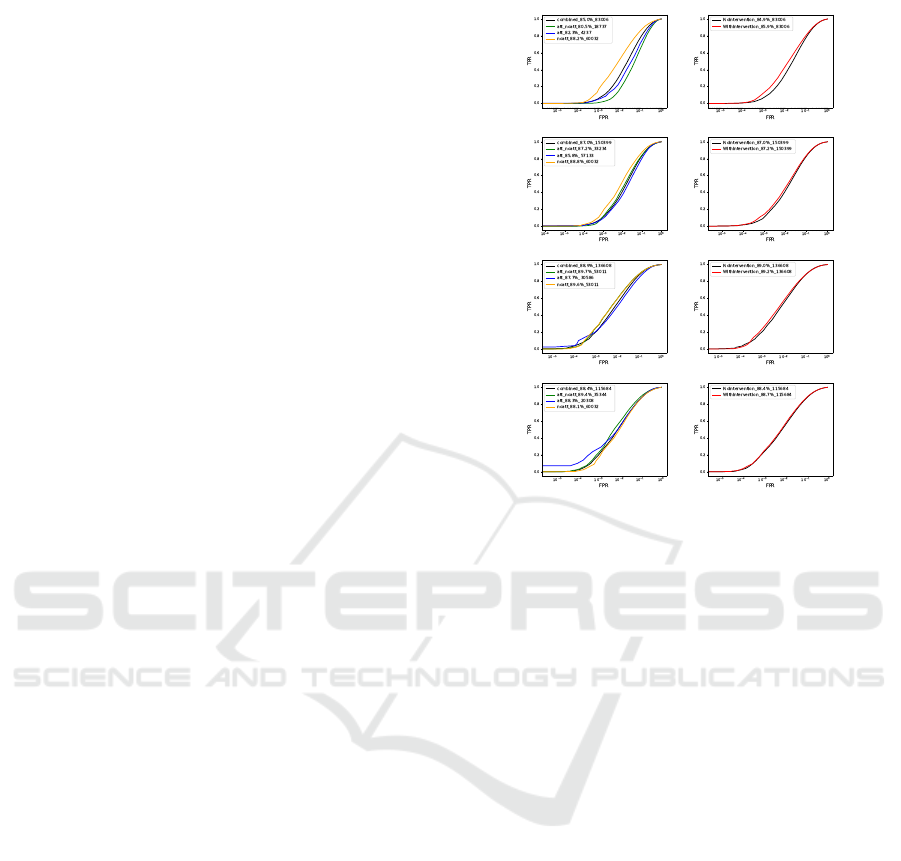
On picking any of the left 4 ﬁgures in 7, for

CelebA dataset, we see the blue line with att-att con-

ﬁg, the green with att-noatt conﬁg, and ﬁnally yel-

low with noatt-noatt conﬁg. The black line repre-

sents, the case where all three conﬁgurations co-exist

in the data i.e. the data is now mixed. As it is observ-

able, each conﬁguration can best be operated upon,

VISAPP 2023 - 18th International Conference on Computer Vision Theory and Applications

164

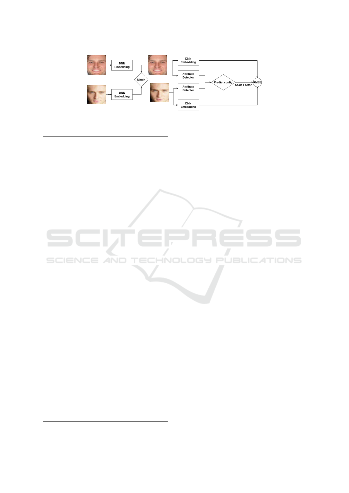
Figure 2: On the left, the regular DNN; Proposed method on the right, where we determine the conﬁg using attribute detector

network, and use mapped scaling-factor(synonymous to unique threshold).RMSE block computes RMSE between two em-

beddings and multiplies with the scaling factor.

Algorithm 1: Conﬁg-speciﬁc operating point.

Require: N face image pairs to match

binT hresh ←Threshold per conﬁg/bin inferenced

from large test-set

ta1 ← 0 (Facial attribute yes/no for the ﬁrst image)

ta2 ← 0 (Facial attribute yes/no for the second im-

age)

probeImage ← f irstimage f rompair

galleryImage ← secondimage f rompair

con f ig ← None (Placeholder for att-att, att-noatt,

noatt-noatt)

getT hresh ← None (picks and returns appropriate

threshold from binThresh for a given conﬁg)

matchDist ← None (RMSE distance between im-

age pair)

t1 ← None (Face template generated by DNN for

image 1)

t2 ← None (Face template generated by DNN for

image 2)

thresh ← None (Threshold returned by getThresh

for a given conﬁguration)

predict ← None (Final genuine impostor predic-

tion by matching function)

Ensure: i = 0, 1...N matching pairs

while N ̸= 0 do

t1 ← DNNEmbeddingGenerator(probe)

t2 ← DNNEmbeddingGenerator(gallery)

matchDist ← RMSE(t1, t2)

ta1 ← FacialAttributeDetectorYesNo(t1)

ta2 ← FacialAttributeDetectorYesNo(t2)

if ta1 = ta2 = 1 then

con f ig ← att − att

thresh ← getT hresh(con f ig, binThresh)

else if ta1 = 0 and ta2 = 1 then

con f ig ← noatt − noatt

thresh ← getT hresh(con f ig, binThresh)

elseta1 = ta2 = 0

con f ig ← noatt − noatt

thresh ← getT hresh(con f ig, binThresh)

end if

predict ← getPredict(thresh, matchDist)

end while

with the knowledge of the conﬁguration. Refer to ﬁg-

ure 2 that explains the same. But how do we deter-

mine if the difference in distribution is induced by

the attribute and not a generic sampling distribution

difference? For this, we cite (Terh

orst et al., 2020a)

where it is shown that the state-of-the-art embedding

FaceNet embedding, has tremendous attribute predic-

tive power, and we use this evidence to back our ex-

perimental setup.

Please note that while preparing the graph 7 we

have made the following assumption: We have elimi-

nated the transparent eyeglasses, and let only the dark

glasses remain to avoid within-class variance).

We have further analyzed the impact of the pose

in the dataset to ensure we have no biased results. No

impact of the pose.

3.1.1 Embedding Used and Choice of Facial

Attributes for This Methodology

The embeddings used to demonstrate this technique

are InceptionResnetV1 pretrained on VGGFace2 (the

dataset has been removed from publicly available ofﬁ-

cial page. Tested on licensed personal copy) as made

available by FaceNet (Schroff et al., 2015), Arcface

model pre-trained on MS1M (Guo et al., 2016), Mag-

face (Meng et al., 2021) model pre-trained on MS1M

dataset.

The choice of attributes of this methodology is the

same as that discussed in the section section 2.3.

3.1.2 Scaling the in-Between Distribution Mean

While the above section offers an insight to operate

individually at each scale, the mechanism to do the

same is detailed below.

∀x

∈ X

where c is conﬁguration in question perform

− µ

(1)

where µ

is the Genuine mean, and µ

is the impos-

tor mean deﬁned for each of the conﬁguration c i.e.

On Attribute Aware Open-Set Face Veriﬁcation

165

att-att, noatt-att, noatt-noatt (for the rest of the pa-

per, please assume att= attribute present. noatt = at-

tribute absent i.e. no att) by passing a statistically rel-

evant huge number of pairs through the trained net-

work. Conceptually we are just zero-centering all

the genuine mean and using the inter-class mean dis-

tance as the scaling factor. This operation helps us

keep the threshold constant while scaling the match

distance. The mean-shifting mentioned above as a

conceptual operation lends itself to methods like pa-

rameter search of each of the conﬁguration means

using methods such as Differential Evolution to ﬁnd

conﬁguration-speciﬁc mean. We used the same in us-

ing Scipy’s implementation of the same in graphs.

3.2 Attribute Aware Face Embedding

and Suppression (AAFES)

The primary object as described in the pipeline 3 is to

leverage identity-rich attribute-aware embedding, to

ﬁrst run an attribute detector over (in this paper how-

ever we use available human annotated attribute labels

for experimental robustness). And once the attribute

is known (say eyeglasses) we apply the suppression

vector, which is essentially a mask we have created

that masks out the most sensitive neurons to a given

attribute, (details explained in this section) to zero out

the neurons showing maximal correlation. The algo-

rithms is given here 2. Note FacialAttributeDetecto-

rYesNo in the algorithm, in our experiment is replaced

with available attribute labels. It is to be noted that we

differ from the work (Diniz and Schwartz, 2021), in

that, we perform a correlation analysis of the ﬁnal em-

bedding layer for a streaming validation data, as op-

posed to a lower dimensional representation of hidden

layer analyzed through images in the cited work.

The details of how the suppression vector is cre-

ated is the focus of the next two subsections

3.2.1 Motivation

We adopted a variation to the quantile streaming anal-

ysis as was used in (Fong and Vedaldi, 2018). We de-

viate from the cited work in that, we gather the acti-

vations of a given neuron (in our case, the embedding

layer neurons) by passing the validation data into the

model, and correlating it with the attribute label of the

image, as opposed to performing quantile analysis on

the same.

Algorithm 2: Algorithm to execute suppression of attribute-

aware embedding.

Require: N image pairs to match

threshold ← Threshold determined by inferencing

embedding over large test-set

suppressionVector ← Determined by our method

for a given attribute

ta1 ← 0 (Facial attribute yes/no for the ﬁrst image)

ta2 ← 0 (Facial attribute yes/no for the second im-

age)

t1 ← None (Face template generated by DNN for

image 1)

t2 ← None (Face template generated by DNN for

image 2)

predict ← None (Final genuine impostor predic-

tion by matching function)

Ensure: i = 0, 1...N matching pairs

while N ̸= 0 do

t1 ← DNNEmbeddingGenerator(probe)

t2 ← DNNEmbeddingGenerator(gallery)

ta1 ← FacialAttributeDetectorYesNo(t1)

ta2 ← FacialAttributeDetectorYesNo(t2)

if ta1 = 1 then

t1 ← t1 ⊙ suppVector

else

t1 ← t1

end if

if ta2 = 1 then

t2 ← t2 ⊙ suppVector

else

t2 ← t2

end if

matchDist ← RMSE(t1, t2)

predict ← getPredict(threshold, matchDist)

end while

3.2.2 Correlating Attribute Label with

Embedding Neurons and Generating

Suppression Vector

Let V be a n1 dimensional embedding, and L be a

n2 dimensional attribute label vector (consisting of 0s

and 1s). Let k be the number of samples in the valida-

tion dataset. For the k samples we now have a n1 × k

matrix of embedding. We also have a k × n2 label-

ing matrix for the k samples. Appending the V

to the

, where i represents a particular sample we get a

n1 + n2 dimensional vector P

for each of k samples.

Using the P matrix of P

vectors we can now form a

covariance matrix as follows:

P,P

∑

i=1

−

P)(P

−

N − 1

(2)

VISAPP 2023 - 18th International Conference on Computer Vision Theory and Applications

166

Figure 3: On the left, the regular DNN; Proposed method on the right, where we determine the conﬁg using attribute detector

network, and use mapped scaling factor.

Since the covariance matrix scales up the correlation

as per the activation values it is dealing with, we per-

form normalized correlation to get the absolute value

of correlation (independent of neuron activation) to

determine which neuron relatively ﬁres most. The re-

lationship between the correlation coefﬁcient matrix,

R, and the covariance matrix, C, is

Ri j =

i j

∗C

j j

(3)

The matrix above can be decomposed as follows:

R =



E M



)×(n

)

(4)

..where E and symmetric E

is the normalized

cross correlation between the embedding, and M and

symmetric M

are normalized cross-correlations be-

tween the embedding vector and the label vector for

a given label. It is the M matrix of shape n1 × n2

that is of interest to us in our suppression. Now

for a given label n2

, we have an embedding cor-

relation vector n1

which is put into 10 bins in the

histogram and index values corresponding to corre-

lation value greater than the second topmost bin and

less than bottom-most 2 bins are chosen. The em-

bedding size we used is size 1792, penultimate to the

fully-connected layer generated embedding of 512 on

the InceptionResnetV1 network (while pre-trained on

VGGFace2, trained on CelebaA by us). It is to be

noted that performing correlation analysis on the ﬁnal

512 embedding too works just as well. Interestingly

while our trained network shows a high correlation for

the discussed attributes, a similar attempt to check the

correlation on the pre-trained embedding of 512 gen-

erated by InceptionResnetV1 on the same discussed

attributes shows that all correlation values like just

about 0.000. Thus showing no strong correlation of

speciﬁc neurons with any attribute, while our embed-

ding does.

3.2.3 Network Used and Training

The network used here is InceptionResnetV1 pre-

trained on VGGFaces2 as made available by FaceNet

(Schroff et al., 2015) as a starting point. The lay-

ers up to ReductionB layer were frozen. Refer Fig-

ure 4 for schematic diagram. This choice of using a

pre-trained network and freezing initial layers was ar-

gued in (Ranjan et al., 2016) to be well suited for face

analysis tasks (attribute detection in our case). The

training was conducted on the Pytorch (Paszke et al.,

2019) platform.

Dropout from the penultimate layer was removed

for ensuring that there is sparsity in the embedding

generated for attribute learning. The remaining lay-

ers were trained on the CelebA dataset with over 40

attributes and over 10,000 identities. Though we fo-

cus on only 4 attributes outlined in the section sec-

tion 2.3, we leverage all the available attribute labels,

to exploit the attribute correlations in the multi-task

setting. Pre-processing is limited to MTCNN (Zhang

et al., 2016) detection, and RGB normalization. At-

tribute and identity accuracy on CelebA dataset as fol-

lows. On attributes accuracies are Smiling - 93% ,

Goatee - 96 %, Heavy-Makeup -90.5% and Mustache

- 96 % on Celeba. Since CelebA doesn’t make an

identity validation set available, we split the training

set to 80-20 ratio, to determine a veriﬁcation accuracy

on a validation set of 91 %. These stats are just to

show that our approach while doesn’t claim a generic

face embedding that can be SOTA ( for instance the

embedding generated by training above has 82% on

LFWA dataset), ﬁnetunes to a speciﬁc dataset con-

taining identity and attribute labeling, and thus enable

both identity and attribute classiﬁcation, and further

using our proposed suppression method enhances the

identity classiﬁcation.

Our multi-task training architecture differs from

(Wang et al., 2017) in that we use the same ﬁnal em-

bedding for the classiﬁcation of both tasks because

we desire a single embedding to encapsulate identity

and attribute information, such that attribute neurons

can later be suppressed. The network is denoted as

f (I;θ), where θ is the parameter set of the deep ar-

chitecture and we use I to denote the training images.

Suppose we have M facial attributes and P face identi-

ties. We model the minimization of the expected loss

On Attribute Aware Open-Set Face Veriﬁcation

167

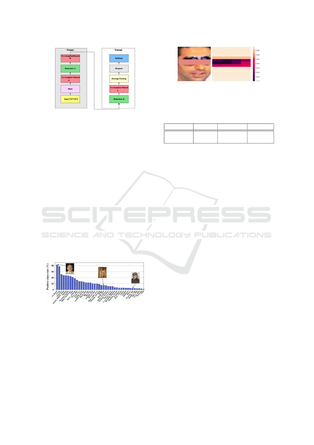
Figure 4: The left half is frozen, while the right half of In-

ceptionResnetV1 is trained.

as follows

Θ, W

, W

= argminL (I;Θ, W

, W

) (5)

where L (I; Θ, W

, W

) is loss function deﬁned of the

task and deﬁned as

L (I;Θ, W

, W

) = L

· f (I; Θ))+L

· f (I; Θ))

(6)

where W

⊆ R

512×2×M

(we have 512x2 here to ac-

commodate a binary classiﬁcation for each attribute,

with CrossEntropy applied over it) and W

⊆ R

512×P

are the learned weights for facial attribute and face

identiﬁcation tasks.

3.2.4 Choice of Attributes in CelebA for AAFES

Method

In addition to section 2.3, for this particular method,

we choose the Smiling attribute because it has more

class balance and hence trains better. The class im-

balance and hence the balance shown by the smiling

attribute is shown in the ﬁg 5

Figure 5: Positive class rate of the smiling attribute is bal-

anced and labeling robust as well.

3.2.5 Sanity Check of Attribute Learning and

Suppression

It is critical that we perform sanity checks if indeed

the attribute is learned by looking at the right regions

of the image, and also if we are really able to isolate

neurons that correlate most with a given face attribute.

For the former, we have performed occlusion exper-

iments, while for the latter we have neuron suppres-

sion to see if face attribute predictions ﬂip.

Figure 6: Pixel level occlusion patch to show the largest

drop in accuracy. The same was performed for Smiling and

bangs.

Table 1: Accuracy before and after suppression in percent-

age for available labels of high conﬁdence from MAAD on

VGGFace2.

Attribute Samples Before (%) After (%)

Smiling 3800 75 0.03

Eyeglasses 4100 98 0.08

Occlusion Experiments: Since our methodology

hinges on the activation of a neuron given a face at-

tribute, in order to ensure that the model has learned

the right regions we performed occlusion experiments

by patching various aspects of images and noticing

drops in classiﬁcation accuracy. In the ﬁg 6 , you’ll

see the patched image on the left and the prediction

conﬁdence plotted on the right. The same was re-

peated for several other attributes such as bangs, and

our subject attribute smiling.

Prediction ﬂip with suppression: In order to check

the effect of suppressing the neurons as deduced

from the distribution of correlation value of embed-

ding neurons, performed the sign ﬂipping experiment,

where I added to the activations a slightly positive

value (about 1 or 1.5) for negatively correlated neu-

rons, and subtracted the same value for activations

with positive correlation, and check the effect of pre-

diction on the accuracy of the attribute. Here is the

accuracy for the attribute before and after the inter-

vention, as applied on VggFace2 dataset (with at-

tribute labels picked up from MAAD annotations of

VGGFace2 (Terh

orst et al., 2020b). The attribute cor-

relation values were derived from activations on a val-

idation set of CelebA, and is being here as shown on

another dataset i.e. VggFace2. Here is “Table 1“

demonstrating the ﬂip in attribute accuracy

4 RESULTS

4.1 Evaluation Methodology

The evaluation method can be summarized as fol-

lows: A standard face veriﬁcation evaluation involves

generating genuine-impostor pairs from probe and

gallery and then splitting the full list of pairs into

train and eval in K-Fold manner. The training set here

VISAPP 2023 - 18th International Conference on Computer Vision Theory and Applications

168

helps determine the optimum threshold for Equal Er-

ror Rate (EER), and the threshold is applied to the

test, to get the test accuracy. The TPR/FPR is gen-

erated from the K-fold test set and averaged. Here

we do the same except that we do it for each of the

conﬁgurations as detailed in section 2.1 i.e. att-att,

att-noatt and noatt-noatt by buckets the probe-gallery

and generating genuine-imposter pair conditioned on

the three conﬁgurations. Detailed steps below:

• Using MTCNN detector to get a clear region

around the face.

• Splitting all images of CelebA or IJB-C (IJB-C

relevant only to eyeglass attribute) dataset into

two bins. The ﬁrst bin has sub-bins, for each fea-

ture, and in turn, each of these bins contains all

the identities who are identiﬁed with that feature.

Similarly a second, has 40 sub-bin, for each fea-

ture, and in turn, each of these bins contains all

identities who are not identiﬁed with that feature

• Half of all the images in the lowest bins are used

for probe and the rest for a test.

• Creating pairs of images from the probe and

gallery set above and iterating through them from

disk with architected Pytorch DataLoader (includ-

ing a change on their open source sampler pro-

gram) to generate a maximum number of pairs,

then generating their embedding, and further their

RMSE distance

• For the generated RMSE and the Gen-

uine/Impostor label assigned as 0/1, a validation

split of 80-20 is done, with K-fold of 10.

• For each training set, a range of thresholds is eval-

uated and for the best threshold, the accuracy is

computed on the validation (20 percent) set.

• This process is repeated for all 10 folds and aver-

age accuracy and TPR/FPR values are reported.

• Since there are a lot more impostor pairs at dis-

posal compared to genuine pairs, the random

genuine-pair-count number of images was sam-

pled from impostor pairs, over 100 trials, and av-

erage accuracy was reported.

4.2 Results for Operating Point

Adjustment by Mean Scaling

4.2.1 Results on CelebA Dataset

As can be seen in the graphs 7 plotted, where each

row represents a particular attribute, the ROC graphs

on the left, show the three individual conﬁgurations

(att/att,att/noatt, noatt/noatt) in color, and the ROC

of the conﬁguration agnostic full pairs of images in

Individual Conﬁguration Full data

Figure 7: Top to bottom: Eyeglass, Heavymakeup, Goatee,

Mustache. ROC plots on left are for individual conﬁgura-

tion; And on the right on full data, with scaling in brown

and; without-scaling in black. The labels on all the graphs

are of the form Accuracy as a number; Intra/inter pair count

and protocol.

black. The image on the right plots the conﬁguration

agnostic graph with and without scaling operation as

described in section 3.1.1. The result clearly shows

that in most conﬁgurations our scaling approach beats

the state-of-the-art at best by 1 % (Eyeglass and goa-

tee). Tables showing accuracies 3 for InceptionRes-

netV1 pretrained on VggFace2 by FaceNet versus

ours.

The table 2 lists the mean and variance before

and after the scaling operation. This shows that once

scaling and shifting are done, all three conﬁgura-

tions end up with GMean (genuine mean) of 0, and

IMean(impostor mean) of 1.

4.2.2 Results on IJB-C Dataset

The IJB-C dataset covers about 3,500 identities with

a total of 31,334 images and 117,542 unconstrained

video frames. We used the occlusion labeling (corre-

sponding to occlusion grid numbers 07 and 09 of IJB-

C https://www.nist.gov/system/ﬁles/documents/2017/

12/26/readme.pdf ) corresponding to the left eye re-

gion and the right eye region, to identify all the

individuals wearing the eyeglass; Similarly, for at-

tribute occluded forehead we used occlusion labels

occ1,occ2,occ3,occ4,occ5 and occ6. We further split

On Attribute Aware Open-Set Face Veriﬁcation

169

Table 2: GMean is the Genuine mean and Gstd is Genuine Standard deviation. Likewise, Imean is Impostor mean.

Att-Att Att-NoAtt NoAtt-NoAtt Full Data

GMean GStd IMean IStd GMean GStd IMean IStd GMean GStd IMean IStd GMean GStd IMean IStd

Eyeglass Before Scale 32.34 7.49 46.5 7.74 42 6.54 53 6.46 38 7.79 55 6.55 38.69 7.87 53.74 6.92

Eyeglass After Scale 8e-05 0.53 0.99 0.54 0.0339 0.59 0.16 0.58 0.00 0.45 1.004 0.38 0.007 0.496 1.00 0.4901

Heavy Makeup Before Scale 33.32 7.30 52.90 7.18 40.16 7.18 55.13 6.25 38.06 7.75 55.46 6.55 38.24 7.53 54.38 6.82

Heavy Makeup After Scale 0.24 0.35 0.12 0.42 0.99 0.35 0.14 0.52 1.03 0.442 4.1 0.37 0.062 0.47 1.00 0.377

Goatee Before Scale 35.0015 7.66 51.98 6.83 38.9 7.54 55.88 5.95 38.97 7.54 55.88 5.95 38.086 7.75 55.25 6.26

Goatee After Scale 9e-05 0.45 1.00 0.40 0.994 0.445 1.002 0.35 0.994 0.44 1.99 0.35 0.003 0.446 1.0011 0.359

Mustache Before Scale 36.4 7.66 52.47 6.58 38.79 7.79 55.85 5.94 38.13 7.78 54.95 6.58 37.86 7.84 54.9 6.39

Mustache After Scale -0.05 0.47 1.00 0.41 0.0004 0.46 1.00 0.39 0.00 0.45 0.99 0.34 -0.009 0.46 0.99 0.37

Table 3: Veriﬁcation accuracy.

Attribute InceptionResnetV1 Ours

Eyeglasses 84.9 85.9

HeavyMakeup 87 87.2

Goatee 88.9 89.3

Mustache 88.5 88.7

the data into bins of att, noatt, att-noatt discussed in

section 2.1 and inferenced the two SOTA approaches,

Facenet, ArcFace (Deng et al., 2019), Magface (Meng

et al., 2021) over it. Our results in “Table 4” shows

that our method section 3.1.2 for eyeglasses attribute

shows a signiﬁcant up to 1 % improvement on ear-

lier SOTAs such as Facenet and ArcFace, while on

the recent SOTA Magface, it equals it, showing that

the SOTA Magface compared to other approaches,

is much more robust in dealing with variation in at-

tributes. For occluded forehead, an attribute which

is more difﬁcult compared to eyeglass (since a lot of

eyeglasses in IJB-C dataset is the see-through eye-

glass providing minimal but deﬁnite occlusion), our

method improves by over 2 % over magface, while

on Facenet it shows 1 % improvement, and ArcFace

shows 0.5% improvement We used to 14900 template

pairs of occluded forehead to report this, and 60000

template pairs of eyeglass attribute to report this.

4.3 Results for Embedding Suppression

Method

4.3.1 ROC Curve for the Dataset with the

Attribute in the Wild

The ROC-curve 10, shows a 3 percentage improve-

ment in the accuracy of veriﬁcation after the suppres-

sion of the attribute.

4.3.2 Qualitative Results

• Figure 9 qualitative demonstrates our results.

• We also analyzed if a RMSE was to be taken only

Figure 8: Top: ROC plots for Facenet on IJB-C dataset.

From the accuracy numbers, one can see the average

of att/noatt/att-noatt protocol is better than combined (in

black) accuracy. Bottom: The plot shows an improvement

in accuracy i.e. 0.5 % increase when mean scaling is done.

cosidering the suppressed neurons, the response

was maximum when pair of images different in

the presence of the attribute

5 CONCLUSIONS

In this paper, we proposed two methods of exploit-

ing attribute information available before matching.

In the ﬁrst case, we determined an ideal operating

point for each conﬁguration (att-att, att-noatt, noatt-

noatt) separately, and used these operating points to

match the pairs at test time (after determining whether

each image in the matching pair has the attribute or

not using attribute detector). To prove the validity

of the same, we used a shift-scale method or param-

eter search using the Differential-evolution method

over learned conﬁguration-speciﬁc genuine-impostor

mean values from training data, and used the plots

showed it beats state-of-the-art veriﬁcation accuracy

on CelebA dataset (for 4 listed attributes) and in case

of IJB-C dataset beats SOTA for a tougher occluded-

forehead attribute while equaling accuracy for eye-

glass attribute. In the second approach, we demon-

VISAPP 2023 - 18th International Conference on Computer Vision Theory and Applications

170

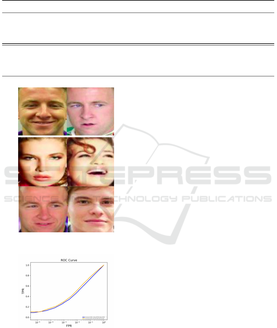
Table 4: Accuracy post att, noatt and att-nott binning individually. Without CSOT refers to current SOTA; CSOT is our

method that uses individual bin thresholds and aggregates the result as explained.

Attribute Model att noatt att-noatt Without CSOT CSOT (Ours)

Eyeglasses Facenet 83.3 87.6 83.0 83.9 84.6

Arcface 88.7 86.6 84.2 85.9 86.4

Magface 95.9 92.3 90.8 93 93.0

Forehead Occlusion Facenet 80.5 85.9 75.7 80.0 80.7

Arcface 84.7 84.2 79.5 82.1 82.7

Magface 93.3 93.0 85.8 88.7 90.7

Figure 9: The top two rows are genuine pairs and the last

row is the impostor pair matched correctly after the suppres-

sion of maximal activation.

Figure 10: The yellow line demonstrates the improvement

in matching after suppression.

strated a way to create attribute-aware embedding and

showed veriﬁcation accuracy can be increased by sup-

pressing the neurons in the embedding correlating

highly with a given attribute, thus showing a method

to suppress the attribute information arguing that sev-

eral applications and methodologies which generate

such embeddings will beneﬁt with the suppression to

increase veriﬁcation accuracy.

REFERENCES

Chen, Z., Liu, F., and Zhao, Z. (2021). Let them choose

what they want: A multi-task cnn architecture lever-

aging mid-level deep representations for face attribute

classiﬁcation. In 2021 IEEE International Conference

on Image Processing (ICIP), pages 879–883.

Deng, J., Guo, J., Xue, N., and Zafeiriou, S. (2019). Ar-

cface: Additive angular margin loss for deep face

recognition. In 2019 IEEE/CVF Conference on Com-

puter Vision and Pattern Recognition (CVPR), pages

4685–4694.

Diniz, M. A. and Schwartz, W. R. (2021). Face attributes as

cues for deep face recognition understanding. CoRR,

abs/2105.07054.

Ferrari, C., Berretti, S., and Bimbo, A. D. (2019). Dis-

covering identity speciﬁc activation patterns in deep

descriptors for template based face recognition. In

2019 14th IEEE International Conference on Auto-

matic Face Gesture Recognition (FG 2019), pages 1–

Fong, R. and Vedaldi, A. (2018). Net2vec: Quantifying and

explaining how concepts are encoded by ﬁlters in deep

neural networks. CoRR, abs/1801.03454.

Gonzalez-Sosa, E., Fierrez, J., Vera-Rodriguez, R., and

Alonso-Fernandez, F. (2018). Facial soft biometrics

for recognition in the wild: Recent works, annotation

and cots evaluation. IEEE Transactions on Informa-

tion Forensics and Security, PP:1–1.

Guo, Y., Zhang, L., Hu, Y., He, X., and Gao, J. (2016). Ms-

celeb-1m: A dataset and benchmark for large-scale

face recognition. In European conference on com-

puter vision, pages 87–102. Springer.

Han, H., Jain, A. K., Shan, S., and Chen, X. (2017). Hetero-

geneous face attribute estimation: A deep multi-task

learning approach. CoRR, abs/1706.00906.

On Attribute Aware Open-Set Face Veriﬁcation

171

Hu, G., Hua, Y., Yuan, Y., Zhang, Z., Lu, Z., Mukherjee,

S. S., Hospedales, T. M., Robertson, N. M., and Yang,

Y. (2017). Attribute-enhanced face recognition with

neural tensor fusion networks. In 2017 IEEE Interna-

tional Conference on Computer Vision (ICCV), pages

3764–3773.

Lu, B., Chen, J., Castillo, C. D., and Chellappa, R.

(2018). An experimental evaluation of covariates

effects on unconstrained face veriﬁcation. CoRR,

abs/1808.05508.

Maze, B., Adams, J., Duncan, J. A., Kalka, N., Miller, T.,

Otto, C., Jain, A. K., Niggel, W. T., Anderson, J., Ch-

eney, J., and Grother, P. (2018). Iarpa janus bench-

mark - c: Face dataset and protocol. In 2018 Inter-

national Conference on Biometrics (ICB), pages 158–

165.

Meng, Q., Zhao, S., Huang, Z., and Zhou, F. (2021).

Magface: A universal representation for face recog-

nition and quality assessment. In Proceedings of the

IEEE/CVF Conference on Computer Vision and Pat-

tern Recognition, pages 14225–14234.

O’Toole, A. J., Castillo, C. D., Parde, C. J., Hill, M. Q., and

Chellappa, R. (2018). Face space representations in

deep convolutional neural networks. Trends in Cogni-

tive Sciences, 22(9):794–809.

Paszke, A., Gross, S., Massa, F., Lerer, A., Bradbury, J.,

Chanan, G., Killeen, T., Lin, Z., Gimelshein, N.,

Antiga, L., Desmaison, A., Kopf, A., Yang, E., De-

Vito, Z., Raison, M., Tejani, A., Chilamkurthy, S.,

Steiner, B., Fang, L., Bai, J., and Chintala, S. (2019).

Pytorch: An imperative style, high-performance deep

learning library. In Wallach, H., Larochelle, H.,

Beygelzimer, A., d'Alch

e-Buc, F., Fox, E., and Gar-

nett, R., editors, Advances in Neural Information Pro-

cessing Systems 32, pages 8024–8035. Curran Asso-

ciates, Inc.

Ranjan, R., Patel, V. M., and Chellappa, R. (2019). Hy-

perface: A deep multi-task learning framework for

face detection, landmark localization, pose estimation,

and gender recognition. IEEE Transactions on Pattern

Analysis and Machine Intelligence, 41(1):121–135.

Ranjan, R., Sankaranarayanan, S., Castillo, C. D., and Chel-

lappa, R. (2016). An all-in-one convolutional neural

network for face analysis. CoRR, abs/1611.00851.

Rudd, E. M., G

unther, M., and Boult, T. E. (2016). MOON:

A mixed objective optimization network for the recog-

nition of facial attributes. CoRR, abs/1603.07027.

Samangouei, P. and Chellappa, R. (2016). Convolutional

neural networks for attribute-based active authentica-

tion on mobile devices. In 2016 IEEE 8th Interna-

tional Conference on Biometrics Theory, Applications

and Systems (BTAS), pages 1–8.

Sankaran, N., Mohan, D. D., Tulyakov, S., Setlur, S., and

Govindaraju, V. (2021). Tadpool: Target adaptive

pooling for set based face recognition. In 2021 16th

IEEE International Conference on Automatic Face

and Gesture Recognition (FG 2021), pages 1–8.

Schroff, F., Kalenichenko, D., and Philbin, J. (2015).

Facenet: A uniﬁed embedding for face recognition

and clustering. CoRR, abs/1503.03832.

Taherkhani, F., Nasrabadi, N. M., and Dawson, J. M.

(2018). A deep face identiﬁcation network enhanced

by facial attributes prediction. CoRR, abs/1805.00324.

Terh

orst, P., F

ahrmann, D., Damer, N., Kirchbuchner, F.,

and Kuijper, A. (2020a). Beyond identity: What infor-

mation is stored in biometric face templates? CoRR,

abs/2009.09918.

Terh

orst, P., F

ahrmann, D., Kolf, J. N., Damer, N., Kirch-

buchner, F., and Kuijper, A. (2020b). Maad-face: A

massively annotated attribute dataset for face images.

CoRR, abs/2012.01030.

Wang, Z., He, K., Fu, Y., Feng, R., Jiang, Y.-G., and Xue, X.

(2017). Multi-task deep neural network for joint face

recognition and facial attribute prediction. In Proceed-

ings of the 2017 ACM on International Conference on

Multimedia Retrieval, ICMR ’17, page 365–374, New

York, NY, USA. Association for Computing Machin-

ery.

Zhang, K., Zhang, Z., Li, Z., and Qiao, Y. (2016). Joint

face detection and alignment using multitask cascaded

convolutional networks. IEEE Signal Processing Let-

ters, 23(10):1499–1503.

VISAPP 2023 - 18th International Conference on Computer Vision Theory and Applications

172