Topological Data Structure: The Fast Marching Example
Sofian Toujja
1
, Thierry Bay
2
, Hakim Belhaouari
1
and Laurent Fuchs
1
1
XLIM, Université de Poitiers, Univ. Limoges, CNRS, XLIM, Poitiers, France
2
CERAMATHS, Université Polytechnique Hauts-de-France, Valenciennes, France
fi
Keywords:
Topological Modeling, Generalized Map, Fast Marching Method, Front Propagation, Jerboa.
Abstract:
This article lies in the field of front propagation algorithms on a surface represented by triangle meshes.
An implementation of the fast marching algorithm using a topological structure, the generalized maps or g-
maps, as the data structure of the mesh is presented. G-maps have the advantage of allowing to store and
retrieve information related to the neighborhood of a cell. In this article, the necessary knowledge about
generalized maps and the fast marching method are reviewed in order to facilitate the understanding of the
proposed implementation and the benefits brought by g-maps as underlying data structure. Then some various
applications of this implementation are presented.
1 INTRODUCTION
This article aims to study the benefits of using a topo-
logical structure as the data structure for mesh algo-
rithms in order to simplify local data access, stor-
age, and modification. This article is part of a larger
project whose objective is to study the volumic ob-
ject’s evolution under constraints. First, the prob-
lem of front propagation on a surface or a volume is
considered. Among the existing algorithms, the fast
marching method (Osher and Sethian, 1988) (Sethian,
1996) has been chosen because it is a well-known al-
gorithm, rather simple to implement, and gives con-
vincing results in a reasonable time. The originality
of the proposed approach lies in the use of a topo-
logical structure, more precisely generalized maps (or
g-maps), as the data structure to handle the computa-
tional data of the algorithms. The use of a topolog-
ical structure such as g-maps allows us to store and
retrieve local information efficiently on the mesh or
in the neighborhood of a cell. Even if performance
must guarantee a practical use, the goal is not to im-
plement the fastest fast marching algorithm but to of-
fer the possibility to extend the fast marching algo-
rithm versatility by using g-maps. In this work, the
software Jerboa (Belhaouari et al., 2014), a topologi-
cal modeler using g-maps, is used to implement the
fast marching algorithm on non-obtuse triangulated
meshes.
As a preamble, important notions for the under-
standing of this implementation are presented. First,
in section 2, the fast marching method applied to non-
obtuse triangulated meshes (Kimmel and Sethian,
1998) is presented. Then, in section 3, the gener-
alized maps (Damiand and Lienhardt, 2014) (Bel-
haouari et al., 2014) are introduced. Finally, in sec-
tion 4, the implementation as well as various practical
uses are detailed.
2 FAST MARCHING METHOD
The necessary principles of the fast marching algo-
rithm to understand the proposed implementation are
presented here. Readers interested in fast march-
ing can refer to (Osher and Sethian, 1988), (Sethian,
1996), (Sethian, 1998) and (Bronstein et al., 2008).
The most common analogy to explain the fast march-
ing method is a forest fire. There may be one or
more sources of the fire. The fire spreads at a differ-
ent speed depending on the land; faster on dry wood
than on wet wood, and not at all on water areas. As
it spreads, the fire consumes the land and does not re-
turn to the already burned areas. The fast marching
algorithm calculates the arrival time of a wave prop-
agating on a manifold by approximating a solution of
the following Eikonal equation at each point:
(
∥
∇T (x)
∥
F(x) = 1
T (x
0
) = 0, F(x) > 0, x, x
0
∈ R
n
(1)
with T the arrival time function, F a given speed
function, x denotes a point and x
0
denotes a given
source point. Based on Dijkstra’s algorithm (Dijk-
stra, 1959), the fast marching algorithm propagates
206
Toujja, S., Bay, T., Belhaouari, H. and Fuchs, L.
Topological Data Structure: The Fast Marching Example.
DOI: 10.5220/0011686800003417
In Proceedings of the 18th International Joint Conference on Computer Vision, Imaging and Computer Graphics Theory and Applications (VISIGRAPP 2023) - Volume 1: GRAPP, pages
206-213
ISBN: 978-989-758-634-7; ISSN: 2184-4321
Copyright
c
 2023 by SCITEPRESS – Science and Technology Publications, Lda. Under CC license (CC BY-NC-ND 4.0)

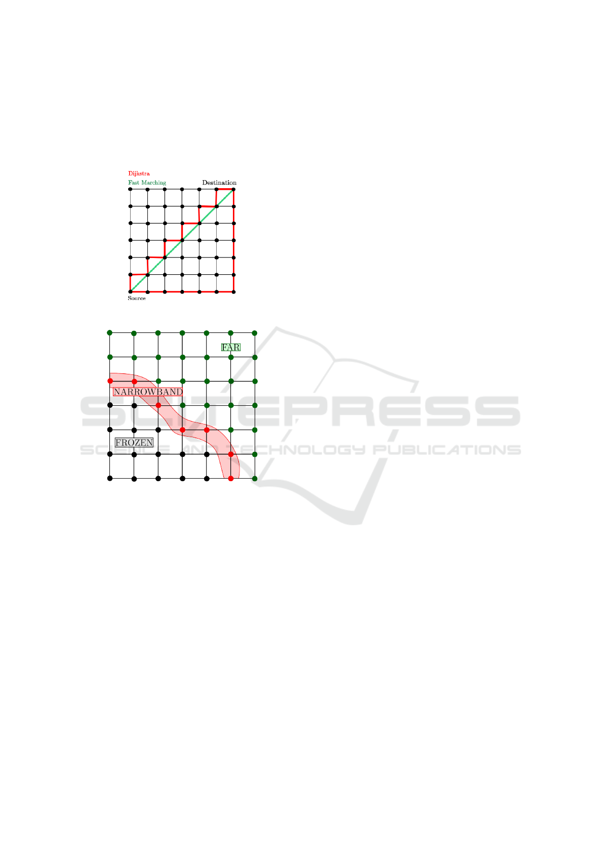
through neighboring vertices. On a surface, fast
marching allows to virtually get rid of the edges and
cross the faces as can be seen in Figure 1. If F(x) =
1, ∀x ∈ R
n
then this method can be used to estimate
the intrinsic distance between two vertices on a man-
ifold.
Figure 1: Dijkstra and fast marching.
Figure 2: Illustration of fast marching propagation.
Initially applicable on an orthogonal n dimen-
sional regular grid (Sethian, 1996), the algorithm was
later extended to triangulated meshes (Kimmel and
Sethian, 1998). The vertices of the mesh have a state
among three states depending on their position rela-
tively to the wave front:
- frozen: the wave front has already passed over the
vertex. An arrival time has been calculated and
does not change anymore.
- narrowband: the wave front is currently on the
vertex. An estimate of the arrival time has been
calculated but may still change.
- far: the wave front has not yet reached the vertex.
Its arrival time from the source is still unknown
and set to a value representing the infinite value.
Figure 2 illustrates the propagation and the dif-
ferent states of a vertex. The propagation goes from
“frozen” vertices to “far” ones. The “narrowband”
represents the current front of the propagation.
Initially, the sources are in the state “frozen” and
their front arrival time is “0”. The other vertices are in
the state “far” and their front arrival time is set to in-
finite value. Each vertex of the mesh has information
on the velocity of the front at this point. Basically,
the algorithm selects the “narrowband” vertex with
the minimal arrival time, set it to “frozen” and calcu-
lates an arrival time estimation for its neighbors and
put them into the “narrowband” state. It loops until
all the vertices are “frozen”, see Algorithm 1. For this
algorithm, accessing the neighbouring information is
one of the key problems. This point motivates the
use of a topological structure which efficiently gives
access to neighbouring elements containing the nec-
essary information.
3 GENERALIZED MAPS
A generalized map (or g-map) is a topological struc-
ture representing, as a graph, the topology of a man-
ifold (orientable or not) by its boundaries (B-rep)
(Damiand and Lienhardt, 2014). Their definition is
homogeneous in all dimensions, avoiding having to
take into account particular cases when developing
dimension-homogeneous algorithms. G-maps repre-
sent structured objects by highlighting the adjacency
relations between the different composing elements.
It is interesting to note that g-maps guarantee us a
topological consistency through the respect of some
constraints, see (Belhaouari et al., 2014). Relations
with other topological structures can be found in
(Lienhardt, 1991).
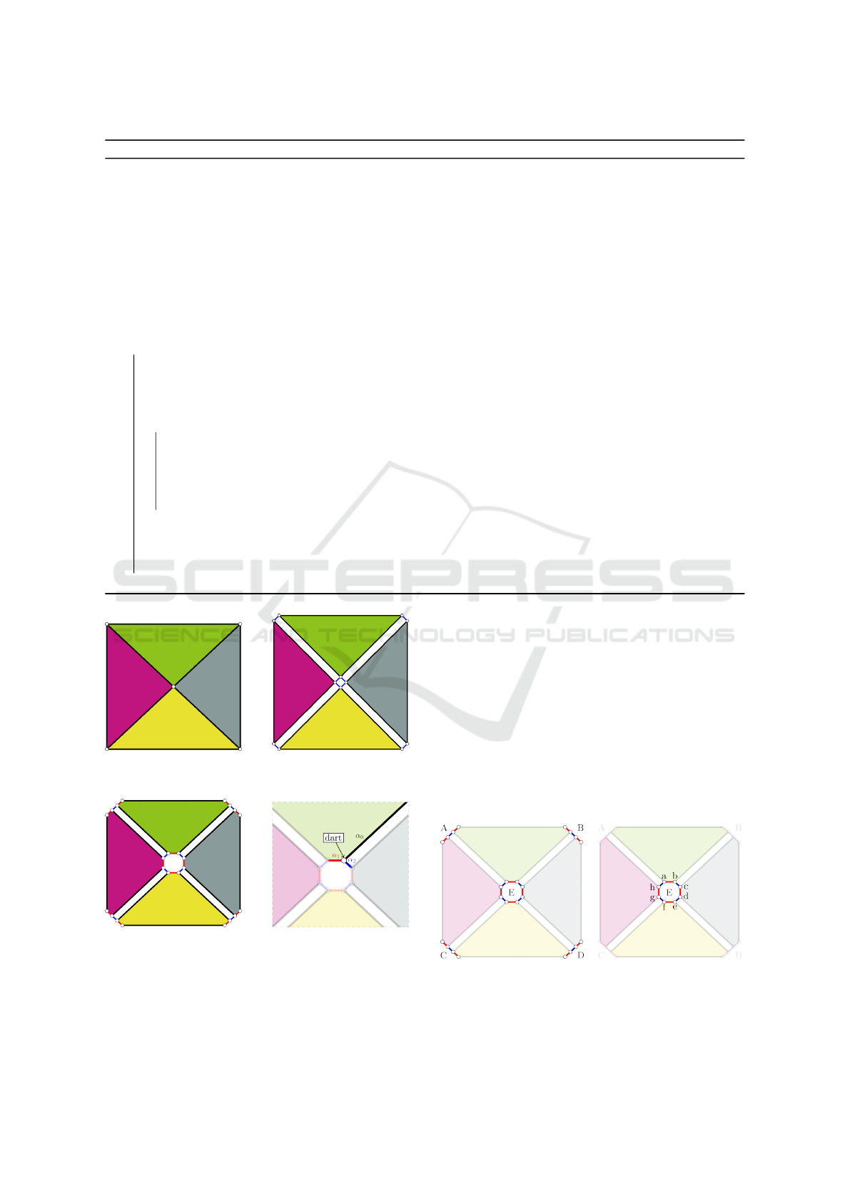
3.1 Construction
G-maps can be constructed intuitively by successive
decomposition of a manifold into cells of decreasing
dimensions. For a manifold of dimension 2, each face
is composed of a set of edges, and each edge is com-
posed of two darts. As darts are atomic elements, the
decomposition stops here. The g-map in Figure 3c
is obtained. The adjacency relations between the dif-
ferent cells are represented by the notation α
i
with i
the dimension of the two connected cells: two faces
(cell of dimension two) are connected by a α
2
link (in
blue in Figure 3d), two edges by a α
1
link (in red),
two vertices by a α
0
link (in black), and two cells of
dimension n by a α
n
link.
Topological Data Structure: The Fast Marching Example
207

Algorithm 1: Fast marching on a non-obtuse triangulated mesh (Bronstein et al., 2008).
Data: a non-obtuse triangulated mesh X, the source x
0
Result: the front arrival time starting from x
0
to all other vertices d : X → R
1 foreach vertex x ∈ X do d(x) ← ∞;
2 d(x
0
) ← 0;
3 /* the arrival time is 0 */
4 Fr ← x
0
;
5 /* list of all frozen vertices */
6 Nb ← N (x
0
);
7 /* vertex priority queue narrowband */
8 Fa ← X \ (Fr ∪ Nb);
9 /* list of all far vertices */
10 while Fr ̸= X do
11 /* while all vertices are not frozen */
12 x
min
← argmin
x∈Nb
d(x);
13 /* The minimal arrival time vertex in Nb */
14 /* estimate the triangles that share the vertex x
min
*/
15 foreach triangle (x
min
, x
2
, x
3
) ∈ {x
min
∈ Nb, x
2
∈ X , x
3
∈ Fr
c
} do
16 /* for all triangles (x
min
, x
2
, x
3
) such as x
3
is not frozen */
17 Nb ← Nb ∪ x
3
;
18 /* x
3
is narrowband */
19 U pdate(x
min
, x
2
, x
3
);
20 /* estimate d(x
3
) from d(x
min
) and d(x
2
) */
21 end
22 /* x
min
is frozen */
23 Nb ← Nb \ x
min
;
24 Fr ← Fr ∪ x
min
;
25 end
(a) Geometric representa-
tion.
(b) Adjacent faces.
(c) G-map obtained. (d) Zoom on dart and rela-
tions.
Figure 3: G-map by successive decompositions.
3.2 Orbits
An orbit is a sub-graph of a g-map. It is a set of darts
that can be reached via a list of defined relations and a
dart to which it applies. It is noted ⟨α
x
, α
y
, . . .⟩(d) with
d the optional application dart. If no application dart
is mentioned, an orbit type is obtained. It selects all
subgraphs corresponding to the set of given relations,
see Figure 4a. If the application dart is specified, an
instance of orbit is obtained, see Figure 4b. In these
two cases, usually the same word “orbit” is used to
designate an orbit type or an instance of orbit.
(a) Orbit type:
⟨α
1
, α
2
⟩
(b) Orbit instance:
⟨α
1
, α
2
⟩(a)
Figure 4: G-map orbits.
GRAPP 2023 - 18th International Conference on Computer Graphics Theory and Applications
208

In Figure 4b, the orbit ⟨α
1
, α
2
⟩ starts on dart “a”
and only α
1
and α
2
are followed. It is interesting to
note that, for example, in Figure 4b: ⟨α
1
, α
2
⟩(a) =
⟨α
1
, α
2
⟩(δ) with δ ∈ {b, c, d, e, f , g, h}.
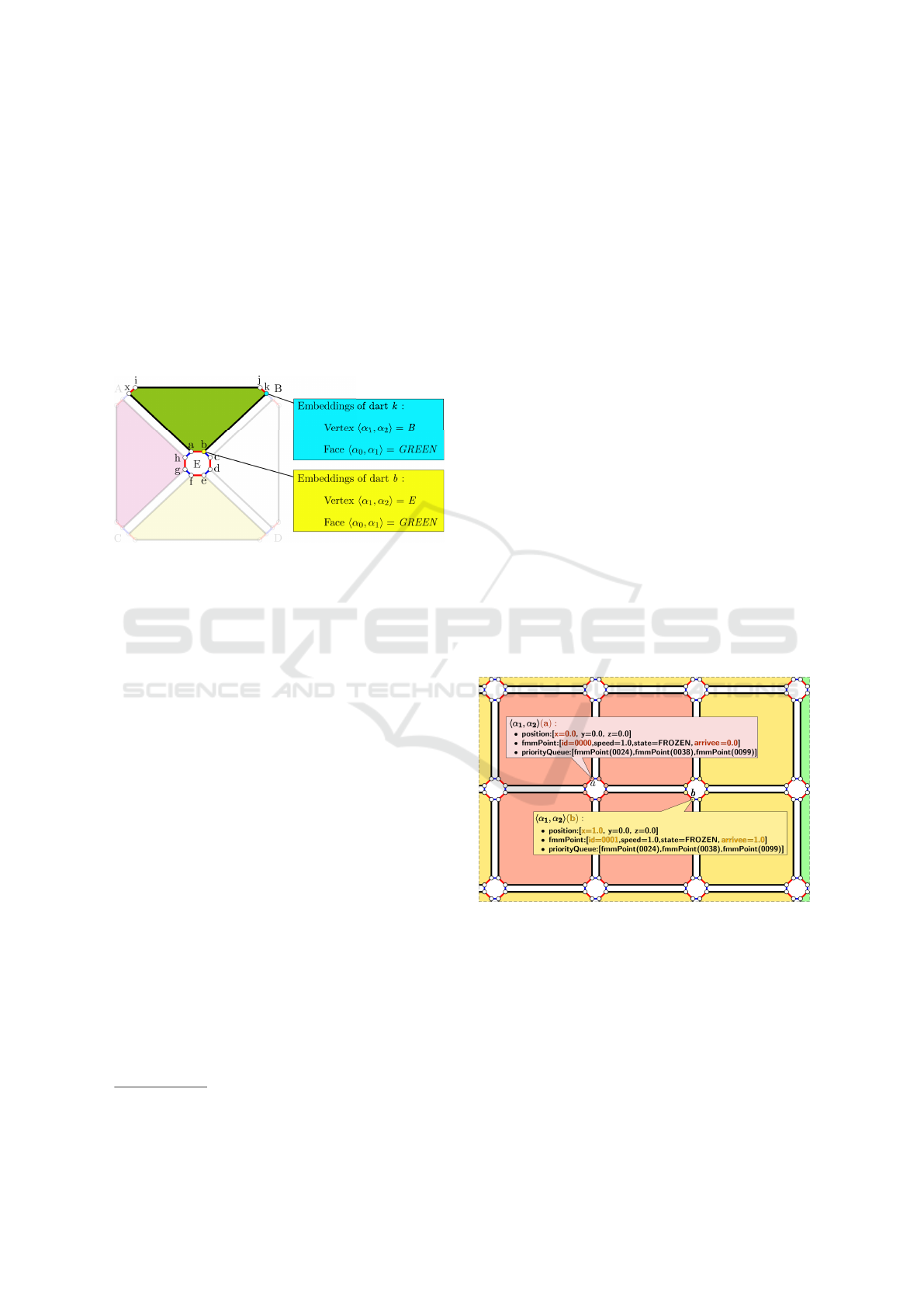
3.3 Embeddings
Properties called “embeddings” can be added to a g-
map. They are defined by a name, an orbit to which
it applies, and a value. The embeddings allow us to
store the information required for the fast marching
algorithm.
Figure 5: Several embeddings.
In Figure 5, the details of the embeddings of two
darts “k” and “b” are highlighted. Both darts have
the same value “GREEN” for the embedding “Face”,
giving the color of a ⟨α
0
, α
1
⟩ orbit. Similarly, the two
darts have different values for the embedding “Ver-
tex”, giving the name of a ⟨α
1
, α
2
⟩ orbit. For one em-
bedding associated with an orbit, the darts in this orbit
have the same embedding value. For example, for the
“Face” embedding, darts “b” and “k” can not have dif-
ferent values. The embedding consistency is handled
via Jerboa: the embedding is shared for all the darts
in the same orbit and the access time is optimal.
4 IMPLEMENTATION
The Jerboa software
1
is used to implement the fast
marching algorithm with a g-map. The main ideas are
to use the embeddings and translate the fast marching
algorithm into Jerboa’s rules (Belhaouari et al., 2014).
The following examples are done in a 3 dimension
generated modeler.
4.1 Jerboa
Jerboa allows us to perform operations on the g-map
through a graph rewriting rule language. Moreover,
1
https://xlim-sic.labo.univ-poitiers.fr/jerboa/ and https:
//xlim-sic.labo.univ-poitiers.fr/logiciels/Jerboa/
Jerboa provides a topological inconsistency detec-
tion during the creation of these new operations (Bel-
haouari et al., 2014) (Ben Salah et al., 2017).
Jerboa carries out the following features:
- Access local information of the g-map via opera-
tors of selection of neighborhood cells (the neigh-
boring faces, the neighboring vertices, etc).
- Create, modify, and associate embeddings with
different orbits.
- Check the consistency of the operations.
- View the created operation in a generated modeler
of the selected dimension.
4.2 Embeddings for Fast Marching
All the vertices (i.e. the orbit: ⟨α
1
, α
2
, α
3
⟩) store in-
formation about their distance from the front, their
state among {frozen, narrowband, far} and the front
speed over them. The whole connected component
(i.e. the orbit: ⟨α
0
, α
1
, α
2
, α
3
⟩) shares a priority queue
containing the “narrowband” vertices sorted by in-
creasing distance. Hence, the g-map structure by it-
self is able to contain all the needed information. Fig-
ure 6 depicts these embeddings on a surface on which
the fast marching is being applied. Each vertex (i.e the
orbit: ⟨α
1
, α
2
, α
3
⟩) has information. The connected
component (i.e the orbit: ⟨α
0
, α
1
, α
2
, α
3
⟩) has a prior-
ity queue, here empty, accessible from each vertex.
Figure 6: Embeddings used for the implementation of fast
marching
4.3 Operations
In Jerboa, operations on g-maps are modeled by rules
that are implemented by graph transforms. The fol-
lowing list of created operations (or rules) changes the
value of the embeddings in the g-map.
- FMMInit ⟨α
0
, α
1
, α
2
, α
3
⟩ initializes the algorithm
for the connected component. A fmmPoint with
Topological Data Structure: The Fast Marching Example
209

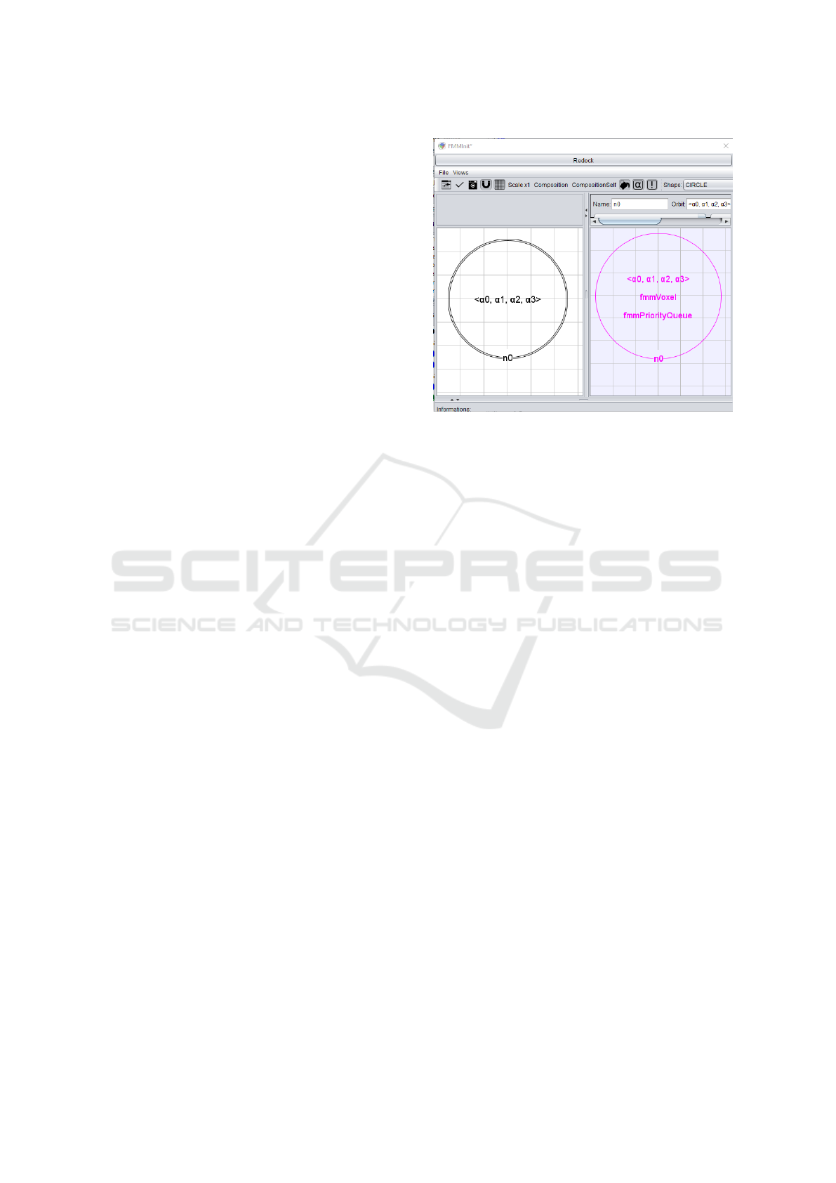
the default values (distance = ∞ ; state = FAR ;
speed = 1) is created for each vertex. The priority
queue is initialized to be empty.
- FMMSetStart ⟨α
1
, α
2
, α
3
⟩ The selected vertices
become the sources of the propagation (distance
= 0 , state = FROZEN).
- FMMMeshComputeFace ⟨α
0
, α
1
, α
3
⟩ for a vertex
in a triangular face, computes the distance based
on the face’s other two points.
- FMMMeshUmbrella performs FMMMeshCom-
puteFace on all faces that share the vertex The
chosen distance is the smallest.
- FMMMeshGo ⟨α
0
, α
1
, α
2
, α
3
⟩ Uses the previous
rules to apply fast marching.
Figure 7 illustrates the definition of the rule
“FMMInit” in Jerboa’s editor. Both circles, called
“nodes”, represent a set of darts. The left one rep-
resents the darts on which the rule applies, here all
the darts in the connected component, i.e in the or-
bit: ⟨α
0
, α
1
, α
2
, α
3
, ⟩. Restrictions can be added in
this node to select darts that follow a specific pattern:
a face, a vertex, a specific geometry such as triangular
faces, and many others, see (Belhaouari et al., 2014).
The right node represents the result of the rule. The
g-map topology is not changed here, so the right node
is similar to the left node, but the value of the embed-
ding “FMMPoint” is changed to return a new FMM-
Point object with some default values (distance = ∞ ;
state = FAR ; speed = 1). Through this notation, once
this rule is applied to a mesh, Jerboa will browse the
whole connected component and affect the values of
FMMPoint for all the vertices. See (Belhaouari et al.,
2014) for other examples of Jerboa rules. It is im-
portant to note that these rules are the only develop-
ment needed to perform fast marching on triangular
meshes. Hence, Jerboa prevents from having to deal
with boilerplate code and allows to focus on the algo-
rithm itself.
4.4 Algorithms
The implementation of the fast marching method on
triangle meshes described by Kimmel & Sethian algo-
rithm (Kimmel and Sethian, 1998) (see Algorithm 1)
on g-maps with Jerboa has been done. It represents
about one hundred line of code in Jerboa script lan-
guage. As a matter of example, the exact Jerboa code
corresponding to the update function (l. 19 in Algo-
rithm 1) is given in Algorithm 2.
Figure 7: FMMInit operation in Jerboa editor.
4.5 Results
This section presents various applications of the fast
marching algorithm using the rules presented in the
previous section.
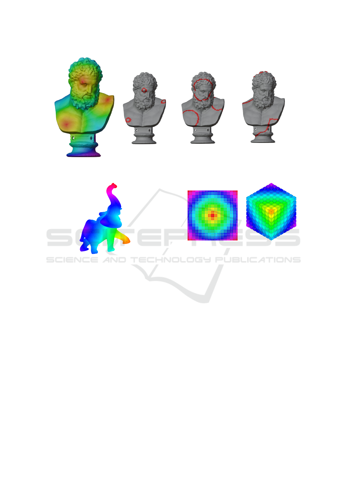
Figure 8a illustrates the application of the fast
marching algorithm using three propagation sources.
The color gradient goes from red (close to the source)
to purple. Figures 8b, 8c, and 8d represent the propa-
gation on the mesh at specific times. Red contours are
isochrones. Reminding equation (1), Γ
t
is the closed
curve representing the set of points located at distance
t from the source (Sethian, 1998). Figure 8d high-
lights the handling of topological modifications of this
approach. The contours merge and continue to prop-
agate.
4.6 Comparison with an Existing
Solution
Although performance in execution time is not our
goal, a comparison has been made with the MATLAB
toolbox developed by G. Peyré (Peyre, 2009), which
is often cited in other works on this topic. The com-
parison has been realized on the same computer in the
same context for both implementations.
The numerical values obtained are equal to the re-
sulting ones from the toolbox. To apply fast marching
with a single source (always the same source) on the
mesh in Figure 9 and display the result, the average
time of the toolbox is 0.4637 seconds versus 6.0843
seconds for this first Jerboa implementation. This dif-
ference reflects the reverse of the gain in consistency
and abstraction brought by the topological structure.
It is quite important to remember that, without even
GRAPP 2023 - 18th International Conference on Computer Graphics Theory and Applications
210

(a) Gradient color
(b) T (x) = 1 (c) T (x) = 5 (d) T (x) = 10
Figure 8: Fast marching with multiple sources.
Figure 9: Comparison mesh (∼ 300 000 darts).
mentioning obvious optimisation improvements, the
development of these rules in Jerboa is quite straight-
forward as Jerboa is handling boilerplate develop-
ments (to store, access, and maintain consistency of
the data, or visualize the results). This methodology
allows to focus on the algorithm and to easily explore
variants in future works (unstructured mesh in arbi-
trary dimension).
4.7 Fast Marching on Regular Volume
Grids
As g-maps are defined homogeneously in any dimen-
sion, this allows us to realize a unique fast marching
rule for both 2D and 3D regular orthogonal grids, see
Figure 10. Moreover, for regular grids this implemen-
tation extends to any desired dimension. Obviously,
for all dimensions, the velocity field can be variable
to add local zones where the front velocity is strongly
penalized.
Figure 10: Same unique rule is used to apply fast marching
on 2D and 3D orthogonal regular grids.
4.8 Fast Marching and Contour
Detection
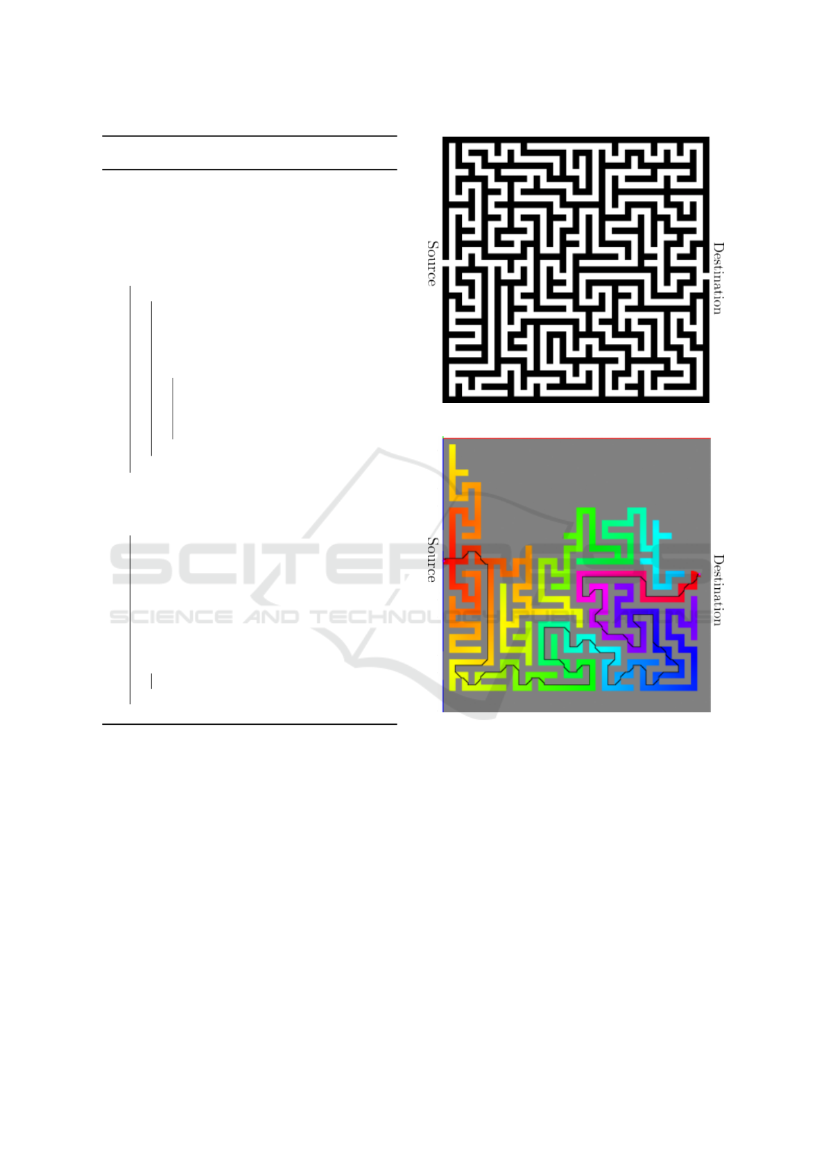
As a playful application, fast marching can find the
shortest path in a maze, see Figure 11. For this pur-
pose, a 2-dimensional grid was created, on which we
have assigned a vertex of the g-map to each pixel of
the maze image. The front velocity on a vertex is pro-
portional to the intensity of the corresponding pixel
(black pixel = low velocity). Once the g-map is set
with the appropriate velocities, fast marching is ap-
plied until the chosen destination point is reached. We
then backtrack from the destination to the source by
selecting the shortest local distance value at each step.
5 CONCLUSION AND
PERSPECTIVES
This work provides g-maps as a data structure for the
fast marching algorithm to add abstraction with the
view to be able to apply this algorithm in unstructured
meshes in arbitrary dimension. G-maps also allow the
Topological Data Structure: The Fast Marching Example
211

Algorithm 2: FMMMeshGoWithoutInit - Apply fast march-
ing on an already initialized mesh.
Data: a dart b ∈ Ω, with Ω = ⟨α
0
, α
1
, α
2
, α
3
⟩
Result: the distance between the source and
all other vertices
1 /* first iteration on the faces
linked to the source vertices to
feed the priority queue */
2 foreach dart b ∈ Ω do
3 if state(b) = FROZEN then
4 ngbr ← b@0;
5 /* ngbr = dart adjacent to b
by the α
0
relation */
6 if state(ngbr) ̸= NARROW BAND
then
7 FMMMeshU mbrella(ngbr);
8 /* Estimate the distance of
the current point using
all the linked faces */
9 end
10 end
11 end
12 /* browse Ω by using the priority
queue */
13 while Ω. f mmPriorityQueue ̸= empty do
14 FMMPoint currentPoint ←
Ω. f mmPriorityQueue.pop();
15 state(currentPoint) ← FROZEN
/* computes a distance
estimation for the vertices of
the neighboring faces of
currentPoint */
16 foreach
dart ngbr ∈ ⟨α
1
, α
2
⟩(currentPoint) do
17 FMMMeshU mbrella(ngbr);
18 end
19 end
storage and retrieval of personalized information
through embeddings and ease of accessing neigh-
borhoods thanks to the notion of orbits. To illus-
trate these points, a naive implementation of the fast
marching algorithm on regular grids (in arbitrary di-
mension) and on triangulated surfaces is proposed.
This work also shows that embeddings-only algo-
rithms can be implemented through Jerboa graphical
language, which simplifies the development thanks
to its boilerplate management (visualization, embed-
ding consistency, optimal information storing and re-
trieval). Furthermore, both of these choices lead to
multiple future works. Indeed, the simplicity brought
by Jerboa allows to prototype and explore variants
made possible by g-maps. Finally, although perfor-
mance is not the main aspect in our work, it could be
improve by parallelizing the calculation. This work is
(a) Initial maze
(b) Resolve with fast marching
Figure 11: Obstacle detection and shortest path.
part of a larger project aiming at modeling the evolu-
tion of volumes under constraints using a topological
structure as the underlying data structure. We thus
plan to continue the work towards contour prediction
on a surface (Chassagne et al., 2020) and then towards
the modeling of the inside of a contour.
ACKNOWLEDGEMENTS
This research has received financial support from the
region Nouvelle-Aquitaine, for the project JACTUM,
convention N
◦
AAPR2021-2020-11919510.
GRAPP 2023 - 18th International Conference on Computer Graphics Theory and Applications
212

REFERENCES
Belhaouari, H., Arnould, A., Le Gall, P., and Bellet, T.
(2014). JERBOA: A Graph Transformation Library
for Topology-Based Geometric Modeling. In Giese,
H. and König, B., editors, 7th International Confer-
ence on Graph Transformation (ICGT 2014), volume
8571, York, United Kingdom. Springer.
Ben Salah, F., Belhaouari, H., Arnould, A., and Meseure,
P. (2017). A general physical-topological framework
using rule-based language for physical simulation. In
12th International Conference on Computer Graphics
Theory and Application (VISIGRAPP/GRAPP 2017),
volume GRAPP of VISIGRAPP 2017 proceedings,
Porto, Portugal.
Bronstein, A., Bronstein, M., and Kimmel, R. (2008). Nu-
merical Geometry of Non-Rigid Shapes. Springer
Publishing Company, Incorporated, 1 edition.
Chassagne, R., Dambrine, J., and Obiwulu, N. (2020). A
new geometrical approach for fast prediction of front
propagation. Computers and Geosciences, 136.
Damiand, G. and Lienhardt, P. (2014). Combinatorial
Maps: Efficient Data Structures for Computer Graph-
ics and Image Processing. A K Peters/CRC Press.
Dijkstra, E. W. (1959). A note on two problems in connex-
ion with graphs. Numerische mathematik, 1(1):269–
271.
Kimmel, R. and Sethian, J. (1998). Computing geodesic
paths on manifolds. Proceedings of the National
Academy of Sciences of the United States of America,
95:8431 – 8435.
Lienhardt, P. (1991). Topological models for boundary rep-
resentation: a comparison with n-dimensional gener-
alized maps. Computer-Aided Design, 23(1):59–82.
Osher, S. and Sethian, J. A. (1988). Fronts propagating
with curvature-dependent speed: Algorithms based on
Hamilton-Jacobi formulations. Journal of Computa-
tional Physics, 79(1):12–49.
Peyre, G. (2009). Toolbox fast marching.
Sethian, J. A. (1996). Theory, algorithms, and applications
of level set methods for propagating interfaces. Acta
Numerica, 5:309–395.
Sethian, J. A. (1998). Fast marching methods. SIAM Re-
view, 41:199–235.
Topological Data Structure: The Fast Marching Example
213