
Thompson Sampling on Asymmetric α-stable Bandits
Zhendong Shi, Ercan E Kuruoglu and Xiaoli Wei
Data Science and Information Technology Center, Tsinghua-Berkeley Shenzhen Institute, Tsinghua University SIGS, China
Keywords:
Thompson Sampling, Multi-Armed Bandit Problem, Asymmetric Reward, Reinforcement Learning,
α
-stable
Distribution.
Abstract:
In algorithm optimization in reinforcement learning, how to deal with the exploration-exploitation dilemma is
particularly important. Multi-armed bandit problem can be designed to realize the dynamic balance between
exploration and exploitation by changing the reward distribution. Thompson Sampling has been proposed in the
literature for the solution of the multi-armed bandit problem by sampling rewards from posterior distributions.
Recently, it was used to process non-Gaussian data with heavy tailed distributions. It is a common observation
that various real-life data such as social network data and financial data demonstrate not only impulsive but
also asymmetric characteristics. In this paper, we consider the Thompson Sampling approach for multi-armed
bandit problem, in which rewards conform to an asymmetric
α
-stable distribution with unknown parameters
and explore their applications in modelling financial and recommendation system data.
1 INTRODUCTION
Sequential decision-making plays a key role in many
fields, such as quantitative finance and robotics. In
order to make real-time decisions under unknown en-
vironments, decision makers must carefully design al-
gorithms to balance the trade-off between exploration
and exploitation. Many decision algorithms have been
designed and widely used, such as financial decision-
making (Shailesh, 2015) and personalized news rec-
ommendation (Li et al., 2010).
The multi-armed bandits (MAB) have an important
potential in solving the dilemma of exploration and
exploitation in the sequential decision-making prob-
lem in which a fixed limited set of resources must be
allocated between competing (alternative) choices in
a way that maximizes their expected gain. Different
data may require different reward distribution. Over
the years, various reward distribution functions rang-
ing from Bernoulli distribution and Gaussian distri-
bution to sub-exponential family, have been proposed
and corresponding fast processing algorithms such as
UCB-Rad (Jia et al., 2021) (specifically for MAB with
sub-exponential rewards) have been developed.
However, when we design decision-making algo-
rithms for complex systems, the reward distribution
function (such as Bernoulli distribution and Gaus-
sian distribution) is inconsistent with the probabil-
ity distribution which each arm obeys. According
to the research on these complex system data, one
can observe that interactions often lead to heavy-tailed
or power law distributions (Lehmkuhl and Promies,
2020). When dealing with practical problems, we find
that many data (e.g. financial data (Embrechts et al.,
2003) and social mobile traffic data (Qi et al., 2016))
have characteristics such as heavy tail and negative
skewness, which cannot be perfectly described by the
Gaussian distribution. These deviations from Gaus-
sian distribution to more complex and practical reward
distributions allow for the opportunity to develop sig-
nificantly more efficient algorithms than were possible
in the original setting as long as we capture the correct
reward distribution in various real world applications.
Existing machine learning algorithms find it diffi-
cult to deal with the problem of multi armed bandits
with complicated reward distributions. This is because
the probability density of such reward distributions
can not be obtained analytically. When real data has
characteristics such as heavy tails or asymmetry, the
standard algorithms which make conservative statisti-
cal assumptions lead to the choice of wrong arms.
In the past few years, there have been a number of
studies on the MAB problem with heavy tailed distri-
butions (Liu and Zhao, 2011),(Bubeck et al., 2013).
Compared with algorithms that are optimized through
repeated trial and error tuning parameters (such as the
epsilon
-greedy algorithm and UCB algorithm), the
consideration of heavy-tail distributions and the devel-
434
Shi, Z., Kuruoglu, E. and Wei, X.
Thompson Sampling on Asymmetric a-stable Bandits.
DOI: 10.5220/0011684200003393
In Proceedings of the 15th International Conference on Agents and Artificial Intelligence (ICAART 2023) - Volume 3, pages 434-441
ISBN: 978-989-758-623-1; ISSN: 2184-433X
Copyright
c
2023 by SCITEPRESS – Science and Technology Publications, Lda. Under CC license (CC BY-NC-ND 4.0)

opment of algorithms for MAB problems involving
heavy tailed data has provided a much more realis-
tic framework leading to higher performance. These
work (e.g. (Lee et al., 2020)) investigated the best
arm identification of MAB with a general assumption
that
p
-th moments of stochastic rewards, analyzed tail
probabilities of average and proposed different bandit
algorithms, such as deterministic sequencing of ex-
ploration and exploitation (Liu and Zhao, 2011) and
truncated empirical average method (Yu et al., 2018).
Instead of tail probabilities, (Dubey and Pentland,
2019) proposed an algorithm based on the symmet-
ric
α
-stable distribution and demonstrated the success
with accurate assumptions and normalized iterative
process.
α
-stable distributions is a family of distribu-
tions with power law heavy tails, which can provide
with a better reward distribution (Dubey and Pentland,
2019) and can be applied to the exploration of complex
systems. This family of distributions stand out among
rival non-Gaussian models (Chen et al., 2016) since
they satisfy the generalised central limit theorem.
α
-
stable distributions have become state of the art models
for various real data such as financial data (Embrechts
et al., 2003), sensor noise (Nguyen et al., 2019), radi-
ation from Poisson field of point sources(Win et al.,
2009), astronomy data (Herranz et al., 2004), and elec-
tric disturbances on power lines (Karaku¸s et al., 2020).
Motivated by the presence of asymmetric character-
istics in various real life data (Kuruoglu, 2003) and the
success in reinforcement learning and other directions
due to the introduction of asymmetry (Baisero and Am-
ato, 2021), in this work, we propose a statistic model,
for which the reward distribution is both heavy-tailed
and asymmetric, named asymmetric alpha-Thompson
sampling algorithm.
2 BACKGROUND INFORMATION
The multi-armed bandit (Auer et al., 2002) is a theo-
retical model that has been widely used in machine
learning and optimization, and various algorithms have
been proposed for optimal solution when the reward
distributions are Gaussian-distribution or exponential-
distribution (Korda et al., 2013). However, these re-
ward distributions do not hold for those complex sys-
tems with impulsive data. For example, when we
model stock prices or deal with behaviour in social
networks, the interactive data often lead to heavy tail
and negative skewness (Oja, 1981).
2.1 Multi-Armed Bandit Problem
Suppose that there are several slot machines available
for an agent, who can select, for each round one to
pull and record the rewards. Assuming that each slot
machine is not exactly the same, after multiple rounds
of operation, we can mine some statistical information
of each slot machine, and then select the slot machine
that gives the expected highest reward.
Learning is carried out in rounds and indexed by
t
∈ [T ]
. The total number of rounds called time range
T
is known in advance. This problem is iterative, the
agent picks arm
a
t
∈ [N]
and then observes reward
r
a
t
(t)
from that arm in each round of
t ∈ [T ]
. For
each arm
n ∈ [N]
, rewards independently come from
a distribution
D
n
with mean
µ
n
=
E
D
n
[r]
. The largest
expected reward is denoted by
µ
?
=
max
n∈[N]
µ
n
, and
the corresponding arm(s) is(are) denoted as the optimal
arm(s) n
∗
.
To quantify the performance, the regret
R(T )
is
used, which refers to the difference between the ideal
total reward the agent can achieve and the total reward
the agent actually gets.
R(T ) = µ
?
T −
T
∑
t=0
µ
a
t
.
(1)
2.2 Thompson Sampling Algorithm for
Multi-Armed Bandit Problem
There are various exploration algorithms, including
the
ε
-greedy algorithm, UCB algorithm, and Thomp-
son sampling.
ε
-greedy algorithm(Korte and Lovász,
1984) uses both exploitations to take advantage of prior
knowledge and exploration to look for new options,
while the UCB algorithm(Cappé et al., 2013) simply
pulls the arm that has the highest empirical reward esti-
mate up to that point plus some term which is inversely
proportional to the number of times the arm has been
played.
Assuming that for each arm
n ∈ [N]
, the reward
distribution is
D
n
parameterized by
θ
n
∈ Θ
(
µ
n
may
not be an appropriate parameter) and that the parameter
has a prior probability distribution p(
θ
n
), Thompson
sampling algorithm updates the prior distribution of
θ
n
based on the observed reward for the arm
n
, and
then selects the arm based on the derived posterior
probability of the reward under the arm n.
According to the Bayes rule,
p(θ|x) =
p(x|θ)p(θ)
p(x)
=
p(x|θ)p(θ)
R
p(x|θ
0
)p(θ
0
)dθ
0
, where
θ
is the model parameter and
x is the observation.
p(θ|x)
is the posterior distribu-
tion,
p(x|θ)
is likelihood function,
p(θ)
is the prior
distribution and p(x) is the evidence.
Thompson Sampling on Asymmetric a-stable Bandits
435

For each round
t ∈ [T]
, the agent draws the pa-
rameter
ˆ
θ
n
(t)
for each arm
n ∈ [N]
from the posterior
distribution of parameters given the previous rewards
up to time
t −1
,
r
r
r
n
(t −1)
=
{r
(1)
n
,r
(2)
n
,··· ,r
(k
n
(t−1))
n
}
,
where
k
n
(t)
is the number of the arm
n
that has been
pulled up at time t:
ˆ
θ
n
(t) ∼ p(θ
n
|r
r
r
n
(t −1)) ∝ p(r
r
r
n
(t −1)|θ
n
)p(θ
n
).
(2)
Given the drawn parameters
ˆ
θ
n
(t) of each arm, the
agent selects the arm
a
t
with the largest average return
on the posterior distribution, receives the return
r
a
t
,
and then updates the posterior distribution of the arm
action a
t
.
a
t
= arg max
n∈[N]
µ
n
(θ
n
(t))
(3)
We will use the Bayesian Regret (Russo and Van,
2014) for the measurement of the performance in order
to compare with the symmetric case. Bayesian Regret
(BR) is the estimated regret over the priors. Denoting
the parameters over all arms as
θ = {θ
1
,...,θ
N
}
and
their corresponding product distribution as
D =
∏
i
D
i
,
the Bayesian Regret is expressed as:
BR(T, π) = E
θ∼D
[R(T )]
(4)
2.3 α-stable Distribution
An important generalization of the Gaussian distribu-
tion is the
α
-stable distribution, which is often used to
model both impulsive and skewed data. It has a non-
analytic density and therefore, usually is described
with the characteristic function. We say a random vari-
able X is S
α
(σ,β,δ) if X has characteristic function
E[e
iuX
] = exp(−σ
α
|
u
|
α
(1 + iβsign(u)
(
|
σu
|
1−α
−1)) + iuδ)
(5)
where
α
is the characteristic exponent defining the
impulsiveness of the distribution, the parameter
β
cor-
responds to the skewness,
γ
is the scale parameter and
δ
is the location parameter. (See (Embrechts et al.,
2003)).
2.4 Symmetric α-thompson Sampling
In MAB with symmetric
α
-stable reward distributions,
the corresponding reward distribution for each arm
n
is given by
D
n
= S
α
(σ,β = 0,δ
n
)
, where
α ∈ (1,2)
,
σ ∈ R
+
are known in advance, and
δ
n
is unknown
((Dubey and Pentland, 2019)). In this case,
E[r
n
] = δ
n
.
They set a prior Gaussian distribution
p(δ
n
)
over the
parameter
δ
n
. Since the only unknown parameter for
the reward distributions is
δ
n
,
D
n
is parameterized by
θ
n
= δ
n
.
(Dubey and Pentland, 2019) propose two algo-
rithms for Thompson Sampling. One is called Sym-
metric
α
-Thompson Sampling, which is based on the
scale mixtures of normals (SMiN) representation. The
other is called robust Symmetric
α
–Thompson Sam-
pling. It is similar to the basic
α
-Thompson sampling,
except for rejecting a reward when the received reward
exceeds the threshold. This strategy yields a tighter
regret bound than the basic Symmetric
α
-Thompson
Sampling. These algorithms, however, do not apply
for asymmetric α-stable MABs since SMiN represen-
tation does not hold.
3 ASYMMETRIC α-THOMPSON
SAMPLING
Both our algorithm and symmetric
α
-Thompson sam-
pling algorithm are constructed under the framework
of Thompson algorithm. The biggest difference is
the assumed reward distribution. Our corresponding
reward distribution for each arm
n
is given by
D
n
=
S
α
(σ,β,δ
n
), where α ∈ (1, 2).
Suppose x is observed data,
δ
n
is the unknown
parameter, we can obtain the posterior density for
δ
n
from prior distribution through the equation (2). How-
ever, as x is assumed to conform to
α
-stable distribu-
tion, density function
f (x|δ
n
)
is unavailable. (Dubey
and Pentland, 2019) take advantage of the symme-
try of the distribution and achieve the iterative process
through scale mixtures of normals representation. This
method is not applicable when β is not equal to 0.
We solve the sampling from the posterior density
problem through Gibbs sampling, which requires ob-
taining conditional distribution. However, it is chal-
lenging to obtain the conditional distribution of
α
-
stable distribution which was circumvented by intro-
ducing an auxiliary variable leading to a decomposi-
tion proposed by (Buckle, 1995).
Theorem 1.
Let
f : (−∞,0) ×(−
1
2
,l
α,β
) ∪(0,∞) ×
(l
α,β
,
1
2
) → (0,∞)
be the bivariate probability density
function of
ˆ
X and
ˆ
Y , conditional on α, β, σ and δ.
f (x,y|α,β, σ,δ) =
α
|α −1|
exp
−|
z
t
α,β
(y)
|
α
α−1
×
z
t
α,β
(y)
α
α−1
1
|z|
(6)
where z =
x−δ
σ
, η
α,β
=
β(2−α)π
2
, l
α,β
= −
η
α,β
πα
.
t
α,β
(y) =
sin[παy + η
α,β
]
cos[πy]
×
cosπy
cos[π(α −1)y + η
α,β
]
α
α−1
.
(7)
ICAART 2023 - 15th International Conference on Agents and Artificial Intelligence
436

Then
f
is a proper bivariate probability density for
distribution of
(X,Y )
, and marginal distribution of
X
is S
α
(σ,β,δ).
Now we are ready to study Bayesian inference for
the arm
n ∈ [N]
. Suppose that at time
t
, the arm
n
has
been pulled for
k
n
(t)
times and hence we have
k
n
(t)
vectors of rewards
r
r
r
n
(t) = {r
(1)
n
,··· ,r
k
n
(t)
n
}
. Accord-
ing to Theorem 1 and the Bayesian rule, we derive
the posterior density of
δ
n
conditional on
r
r
r
n
(t)
by the
following equation(Buckle, 1995):
p(α,β,σ, δ
n
|r
r
r
n
(t)) ∝
Z
(
α
|α −1|σ
)
k
n
(t)
exp
−
k
n
(t)
∑
i=1
|
z
i
t
α,β
(y
i
)
|
α
α−1
×
k
n
(t)
∏
i=1
z
i
t
α,β
(y
i
)
α
α−1
1
|z
i
|
×p(α,β,σ,δ
n
)dy
(8)
where
z
i
=
r
(i)
n
−δ
n
σ
and
p(δ
n
)
is the prior distri-
bution for
δ
n
. We can simplify the formula further as
α,β,σ are known.
p(δ
n
|α,β, σ,r
r
r
n
,y
y
y
n
) ∝ exp{−
k
n
(t)
∑
i=1
|
z
i
t
α,β
(y
i
)
|
α/(α−1)
}
×
k
n
(t)
∏
i=1
|
z
i
t
α,β
(y
i
)
|
α/(α−1)
×
1
|z
i
|
p(δ
n
)
(9)
Through this formula, we have completed the
method to obtain the posterior distribution under the
assumption of asymmetric α-stable distribution.
In our algorithm we first estimate parameters
α,β,σ
and choose normal distribution as the prior dis-
tribution of
δ
. Suppose that we have a model driven
by the parameter vector
(α,β,δ, σ)
, and that we have
observed
x = (x
1
,x
2
,...,x
n
)
. By taking a set of starting
values we can generate
µ
1
from
π(δ|α
0
,β
0
,σ
0
,x)
,
α
1
from
π(α|δ
1
,β
0
,σ
0
,x)
, and so on continuing to other
parameters thereby performing one iteration producing
the sample
(α
1
,β
1
,δ
1
,σ
1
)
. The prior distribution of
σ
is also taken to be a Gaussian distribution, while the
prior distributions of
α,β
are chosen to follow beta
distribution.
The conditional distributions of
α
-stable parame-
ters are obtained as follows:
p(α
n
|δ,β, σ,r
r
r
n
) ∝ (
α
|α −1|
)
n
exp(−
k
n
(t)
∑
i=1
|
z
i
v
i
|
α
α−1
)×
k
n
(t)
∏
i=1
|
z
i
v
i
|
α
α−1
|
dt
α,β
dy
|
−1
t
α,β
(y
i
)=Φ
i
(r
(i)
n
−δ
n
)
p(α
n
)
(10)
p(β
n
|α,δ,σ,r
r
r
n
) ∝ |
dt
α,β
dy
|
−1
t
α,β
(y
i
)=Φ
i
(r
(i)
n
−δ
n
)
p(β
n
)
(11)
p(σ
n
|α,δ,β,r
r
r
n
) ∝ |
dt
α,β
dy
|
−1
t
α,β
(y
i
)=Φ
i
(r
(i)
n
−δ
n
)
p(σ
n
)
(12)
Algorithm 1: Asymmetric α-Thompson Sampling.
Input:
Arms n
∈
[N], priors
α,β,σ
for each arm,
auxiliary variable y
estimate
α,β,σ
by empirical characteristic function
method and deduce prior distribution p(δ)
for each arms n ∈ [N] do
for each iteration t ∈ [k
n
(t)] do
draw δ
n
(t) from prior distribution
Generate u from a Uniform(0,1)
If
u
<
p(
ˆ
δ
n
(t)|α,β,σ,r
r
r
n
(t)) × p(δ
n
(t)|
ˆ
δ
n
(t))
/(p(δ
n
(t)|α,β,σ,r
r
r
n
(t))p(
ˆ
δ
n
(t)|δ
n
(t)))
then
δ
n
(t + 1) =
ˆ
δ
n
(t)
; otherwise,
δ
n
(t + 1) =
δ
n
(t)
choose the arm that maximizes the reward
r
(t)
n
Update distribution p(δ
n
(t + 1)) by (9)
Update distribution p(α
n
(t + 1)) by (10)
Update distribution p(β
n
(t + 1)) by (11)
Update distribution p(σ
n
(t + 1)) by (12)
3.1 Regret Analysis
Bayesian Regret.
In this section, we provide a for-
mula for the Bayesian Regret (BR) incurred by the
asymmetric α-Thompson Samplings algorithm.
In order to simplify the calculation formula, we in-
troduce the upper bound confidence and lower bound
confidence to show the Bayesian Regret. We gener-
alize the upper and lower confidence bounds on an
arm’s expected rewards at a certain time t (given his-
tory
H
t
): respectively,
U(a, H
t
)
and
L(a,H
t
)
. There
are two properties we want these functions to have, for
some γ > 0 to be specified later:
∀a,t E[[U(a,H
t
) −µ(a,t)]
−
] ≤ γ
(13)
∀a,t E[[µ(a,t) −L(a,H
t
)]
−
] ≤ γ
(14)
Assuming we have lower and upper bound func-
tions that satisfy those two properties, the Bayesian
Regret of Thompson sampling can be bounded as fol-
lows:
BR(T ) ≤2γ ×T ×N+
T
∑
t=1
E[[U(a,H
t
) −L(a,H
t
)]]
(15)
Theorem 2.
Let
N
>1,
α ∈ (1,2)
,
σ ∈ R
+
. As-
sume that
δ
n∈[N]
is uniformly bounded by
M > 0
,
i.e.
δ
n∈[N]
∈ [−M,M]
. Then for a N-armed bandit
with rewards for each arm
n
independently drawn
from
S
α
(β,σ,δ
n
)
, for
ε
chosen a priori such that
ε → (α −1)
−
,
Thompson Sampling on Asymmetric a-stable Bandits
437

BR(T,π
T S
) = O(N
1
1+ε
T
1+ε
1+2ε
)
(16)
Proof.
For all heavy-tailed distributions such as
α
-
stable distributions, variance does not exist, so we need
to build our own controllable
σ
. The key difference
between our BayesRegret and the results from (2) lies
in the moments of
α
-stable distribution. We have for
X ∼ S
α
(σ,0,0), ε ∈ (0, α −1)
E[|X|
(1+ε)
] = C(1 + ε, α)|σ|
(1+ε)/α
(17)
where
C((1 + ε),α) =
2
ε
Γ(
ε
2
)Γ(−
(1+ε)
α
)
α
√
πΓ(−
(1+ε)
2
)
. while
β 6= 0
,
by Proposition 1 in (Kuruoglu, 2001), we have for
X ∼ S
α
(σ,β,0), p ∈ (0,α).
E[|X|
(1+ε)
] = C((1 + ε), α,β)|σ|
(1+ε)/α
(18)
where
C((1 + ε), α,β) =
Γ(1−
(1+ε)
α
)
Γ((−ε))
1
cosθ
(1+ε)/α
×
cos(
(1+ε)θ
α
)
cos(
(1+ε)π
2
)
and θ = arctan(βtan
απ
2
).
Let
x
1
,x
2
,...,x
n
be a real i.i.d. sequence with finite
mean
µ
. Assume for some
ε ∈ (0,1]
,
v ≥ 0
and
u ≥ 0
,
one has E[|X −µ|
1+ε
] ≤ v and E[|X|
1+ε
] ≤ u.
Let
ˆµ
be empirical mean, then for any
δ ∈ (0,1)
,
with probability at least
1 − δ
. One has
ˆµ ≤ µ +
(
3∗v
δ∗n
ε
)
1
1+ε
(Bubeck et al., 2013).
Thus, through the definition of upper bound con-
fidence, lower bound confidence and
γ
, we obtained
γ ≤ 2 ∗NM ∗δ ∗T where |U(a, H
t
)| ≤ M.
T
∑
t=1
E[[U(a, H
t
) −L(a,H
t
)]] ≤ 2 ∗E[
N
∑
n=1
T
∑
t=1
I[A
t
= k]
(
3 ∗v
δ ∗n
ε
)
1
1+ε
]
≤ 2 ∗(
3 ∗C(1 + ε,α,β)
δ ∗n
ε
)
1
1+ε
E[
N
∑
n=1
Z
k
n
(T )
s=0
(
1
s
ε
)
1+ε
ds]
= 2(1 + ε)(
3C(1 + ε,α,β)
δ ∗n
ε
)
1
1+ε
∗(NT)
1
1+ε
(19)
BR(T,π
T S
) ≤ 4
3 ∗C(1 + ε,α,β)
δ
1
1+ε
(NT)
1
1+ε
+ 4NMT
2
δ,
(20)
where
δ ∈ (0,1)
. By choosing suitable
δ
, we obtain
the desired equation (16).
In particular, when β = 0 or β = ±1.
BR(T,β = 0) ≤4
3 ∗
Γ(1−
p
α
)
Γ(1−p)
1
cos(
pπ
2
)
δ
1
1+ε
(NT)
1
1+ε
+ 4NMT
2
δ
(21)
BR(T,β = ±1) ≤4
3 ∗
Γ(1−
p
α
)
Γ(1−p)
(
1
cos(
pπ
2
)
)
p/α
δ
1
1+ε
(NT)
1
1+ε
+ 4NMT
2
δ
(22)
where (21) is consistent with the results obtained in
the symmetric case.
Although the skewness parameter
β
has an impact
on the regret bound, it does not change the upper con-
fidence bound of the regret bound, which is shown in
(16).
4 EXPERIMENTAL STUDIES
In order to show the efficiency and stability of the
asymmetric
α
-TS algorithm in a specific data field, we
will use the
ε
-greedy algorithm, bootstrapped UCB
algorithm, symmetry
α
-TS algorithm and asymmet-
ric algorithm in different data sets for comparative
experiments.
To test the efficiency of asymmetric
α
-TS algo-
rithm, we use synthetic
α
-stable data, stock prices data
and recommendation data as detailed next.
4.1 Synthetic Asymmetric α-stable Data
We generated a simulated data set with 100 arms. We
generated
x
t,a
∈ R
from alpha-stable distributions for
all arms a. The true parameters were firstly simulated
from an alpha-stable distribution with mean 0. The
resulting reward associated with the optimal arm was
0.994 and the mean reward was 0.195. We averaged
the experiments over 100 runs.
This asymmetric data set is generated using the
Chambers-Mallows-Stuck algorithm (Weron, 1996).
We conducted multi-armed bandit experiments with
following benchmarks – (i) an
ε
-greedy agent, (ii)
Boostrapped-UCB agent, (iii) Symmetric
α
-TS and
(iv) Asymmetric
α
-TS. The average value of each arm
is randomly selected, where
α = 1.3
and
σ = 500
re-
spectively of each experiment.
ICAART 2023 - 15th International Conference on Agents and Artificial Intelligence
438
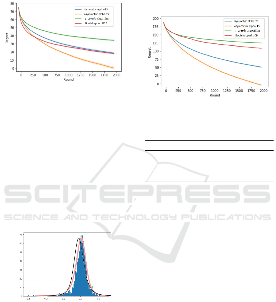
Figure 1: Regret for asymmetric data, the green line is
greedy strategy, blue one is common alpha-TS method, red
one is Bootstrapped UCB while orange line shows our asym-
metric α-TS method.
The test results of the asymmetric data which are
shown in Figure 1 meet our expectations, and the sym-
metric algorithm is worse than our method in time and
space efficiency. Under the assumption that the return
distribution conforms to the asymmetric
α
-stable distri-
bution, we obtain reward each iteration independently
come from the reward distribution.
4.2 Stock Selection
In this experiment, 100 shares listed in Shenzhen Stock
Exchange through Tushare using Python had been
chosen as risk assets, and the stock codes are from
000010.SZ to 300813.SZ. We choose the closed stock
price from 2016/07/01 to 2020/07/18.
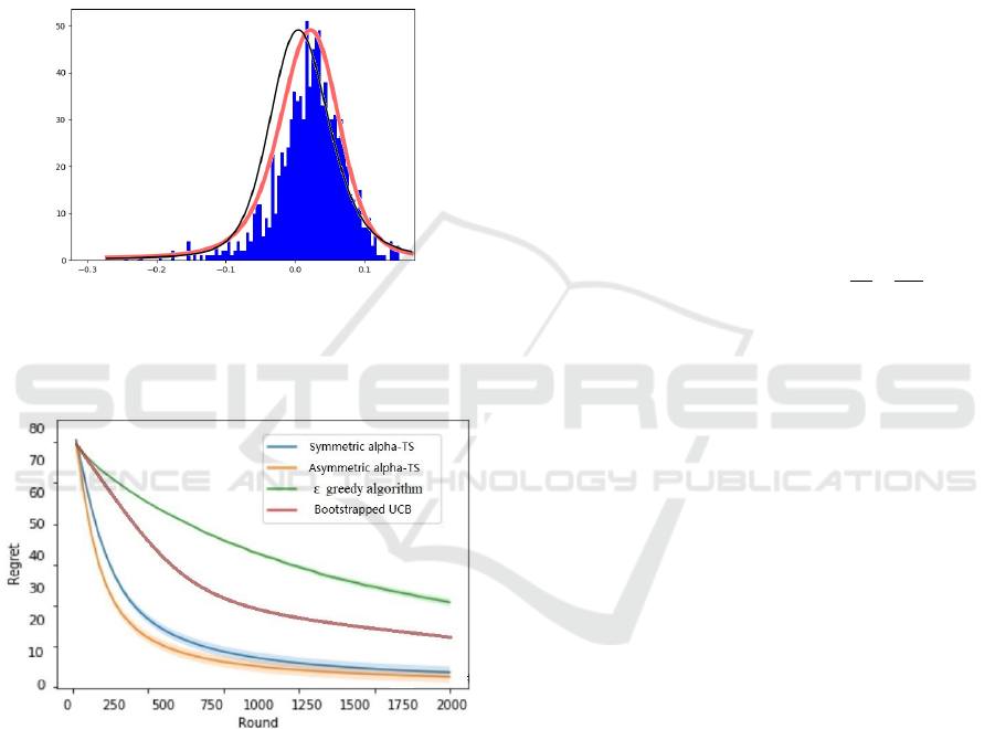
Figure 2: Stock price data, the blue histogram represents
the dataset, the black curve represents the fitted symmetric
α
stable distribution and the red one represents the fitted
asymmetric α stable distribution.
In the financial field, reward distribution can be
regarded as the distribution of return on each stock.
In each iteration, we get the parameters that are more
consistent with the actual distribution under the as-
sumption conditions and the maximum arm obtained
by sampling. The regret tells the difference between
the ideal total reward we can achieve and the total
reward we actually gets.
Figure 3: regret for stock price data, the green line is greedy
strategy, blue one is common alpha-TS method, red one is
Bootstrapped UCB while orange line shows our asymmetric
α-TS method.
Table 1: Comparison of Different Strategies.
Strategy AR SR MaxD
ε −greedy 3.36% 9.2% 3.48%
Boostrapped −UCB 6.47% 8.3% 6.35%
Symmetric −T S 7.76% 17.8% 3.39%
Asymmetric −T S 9.68% 23.5% 3.5%
The performance of our trading strategies are
compared with
ε − greedy
, Boostrapped-UCB and
Symmetric-TS through Annual Return (AR), Sharpe
Ratio (SR), and Maximum Drawdown (MaxD, namely
the maximum portfolio value loss from the peak to the
bottom). The performances of AR, SR, and MaxD. are
shown in Table 1.
We can see the excellent performance of the
asymmetric-TS algorithm from Figure 3 in the field of
stock selection as the log return of stock is consistent
with asymmetric
α
-stable distribution. The regret is
reduced to close to 0, which means that the asymmet-
ric
α
-stable distribution can almost perfectly fit the
distribution of log return of stock prices. Our algo-
rithm also gets the optimal Annual Return (AR) and
the maximum Sharpe Ratio (SR), which means that it
has good profitability and stability.
In order to illustrate the versatility of Thompson
sampling for bandit settings more complicated than
just one original data each time, one may consider
stochastic Stock portfolio selection problems that re-
late to the correlation between actions.
4.3 Recommendation System
Recommendation systems are also common applica-
tions of Multi-armed Bandits. The items to be recom-
mended are modeled as the arms to be pulled. The
Thompson Sampling on Asymmetric a-stable Bandits
439
recommendation system gets a score according to its
own scoring system, and we regard the distribution of
score as our reward distribution. Thus, the main goal
is also to maximize the expected reward achieved after
T times.
In this section, we have utilized two benchmark
datasets (MovieLens 100K) of the real-world in rec-
ommender systems to implement the model practi-
cally. MovieLens 100K contains 100,000 ratings
R ∈ {1,2,3,4, 5}
,
1682
movies (items) rated by
943
users.
Figure 4: Recommendation data, the blue histogram rep-
resents the dataset, the black curve represents the fitted
symmetric
α
stable distribution and the red one represents
the fitted asymmetric α stable distribution.
Figure 5: Regret for recommendation data, the green line is
Bootstrapped UCB, blue one is common alpha-TS method
while orange line shows our asymmetric α-TS method.
Thompson Sampling algorithms learn the rating
distributions of films in few rounds, while
ε −greedy
and Boostrapped-UCB fall into local optima. Figure
5 shows that Thompson Sampling strategy is more
appropriate than
ε
-greedy and UCB strategy in a noise-
free environment. The difference between symmetric
and asymmetric algorithms is not significant, which
may be due to the fact that the movie dataset conforms
to the symmetric situation, or it may be due to the
constrains of dataset rating R ∈ {1,2,3, 4,5}.
5 CONCLUSIONS
In view of the complexity of action/observation space
in many problems, we designed an asymmetric
α
Thompson sampling algorithm using Bayesian infer-
ence for stable distribution and verified the conjecture
through the asymmetric data ,real stock price data and
recommendation data.
Asymmetric
α
-stable algorithm can also be used
to process symmetric data because it has no restric-
tions on
β
, but because it uses complicated Bayesian
inference formula (in the symmetric
α
Thompson algo-
rithm, the iteration from prior distribution to posterior
distribution can be greatly simplified through the char-
acteristics of symmetry and alternative variables), the
iteration speed can not be compared with symmetric
α
Thompson algorithm which can iterate from prior dis-
tribution to posterior distribution immediately under
symmetric conjecture and auxiliary variables.
We develop a regret bound for asymmetric
α
one
in the parameter, action and observation spaces. Our
algorithms only require the existence of bounded 1 +
ε
moment of payoffs, and achieve
O(N
1
1+ε
T
1+ε
1+2ε
)
regret
bound which can be used to determine the rationality
of the data.
Applying the algorithm to stock price returns and
recommendation systems, we demonstrate that asym-
metric stable distribution is a better data model, which
can explain the existence of skewness.
REFERENCES
Auer, P., Cesa-Bianchi, N., and Fischer, P. (2002). Finite-
time analysis of the multiarmed bandit problem. Ma-
chine learning, 47(2-3):235–256.
Baisero, A. and Amato, C. (2021). Unbiased Asymmetric
Actor-Critic for Partially Observable Reinforcement
Learning. The Computing Research Repository.
Bubeck, S., Cesa-Bianchi, N., and Lugosi, G. (2013). Ban-
dits with heavy tail. IEEE Transactions on Information
Theory, 59(11):7711–7717.
Buckle, D. (1995). Bayesian inference for stable distribu-
tions. Journal of the American Statistical Association,
90(430):605–613.
Cappé, O., Garivier, A., Maillard, O.-A., Munos, R., and
Stoltz, G. (2013). Kullback-Leibler upper confidence
bounds for optimal sequential allocation. The Annals
of Statistics, page 1516–1541.
Chen, Y., So, H. C., and Kuruoglu, E. E. (2016). Variance
analysis of unbiased least lp-norm estimator in non-
gaussian noise. Signal Processing, 122:190 – 203.
Dubey, A. and Pentland, A. (2019). Thompson Sampling on
Symmetric alpha-Stable Bandits. International Joint
Conference on Artificial Intelligence.
ICAART 2023 - 15th International Conference on Agents and Artificial Intelligence
440

Embrechts, P., Lindskog, F., McNeil, A., and Rachev, S.
(2003). Handbook of heavy tailed distributions in fi-
nance. Modelling Dependence with Copulas and Appli-
cations to Risk Management. Handbooks in Finance:
Book, 1:329–385.
Herranz, D., Kuruo
˘
glu, E. E., and Toffolatti, L. (2004). An
alpha-stable approach to the study of the P(D) distribu-
tion of unresolved point sources in CMB sky maps.
Astronomy & Astrophysics, 424(3):1081–1096.
Jia, H., Shi, C., and Shen, S. (2021). Multi-armed Bandit
with Sub-exponential Rewards. Operations Research
Letters, 49(5):728–733.
Karaku¸s, O., Kuruo
˘
glu, E. E., and Altınkaya, M. A. (2020).
Modelling impulsive noise in indoor powerline commu-
nication systems. Signal, Image and Video Processing,
14(8):1655 – 1661.
Korda, N., Kaufmann, E., and Munos, R. (2013). Thompson
sampling for 1-dimensional exponential family bandits.
Proceedings of NIPS.
Korte, B. and Lovász, L. (1984). Greedoids-a structural
framework for the greedy algorithm. Progress in com-
binatorial optimization, pages 221–243.
Kuruoglu, E. E. (2001). Density parameter estimation of
skewed/spl alpha/-stable distributions. IEEE Transac-
tions on signal processing, 49(10):2192–2201.
Kuruoglu, E. E. (2003). Analytical representation for pos-
itive /spl alpha/-stable densities. In 2003 IEEE Inter-
national Conference on Acoustics, Speech, and Signal
Processing, 2003. Proceedings. (ICASSP ’03)., vol-
ume 6, pages VI–729.
Lee, K., Yang, H., and Lim, S. (2020). Optimal algorithms
for stochastic multi-armed bandits with heavy tailed
rewards. Advances in Neural Information Processing
Systems, 33:8452–8462.
Lehmkuhl, M. and Promies, N. (2020). Frequency distribu-
tion of journalistic attention for scientific studies and
scientific sources: An input–output analysis. PloS one,
15(11):e0241376.
Li, L., Chu, W., Langford, J., and Schapire, R. E. (2010).
A contextual-bandit approach to personalized news
article recommendation. Proc.of Intl Conf.on World
Wide Web, pages 661–670.
Liu, K. and Zhao, Q. (2011). Multi-armed bandit problems
with heavy-tailed reward distributions. In 2011 49th
Annual Allerton Conference on Communication, Con-
trol, and Computing (Allerton), pages 485–492. IEEE.
Nguyen, N. H., Do
˘
gançay, K., and Kuruo
˘
glu, E. E. (2019).
An Iteratively Reweighted Instrumental-Variable Es-
timator for Robust 3-D AOA Localization in Impul-
sive Noise. IEEE Transactions on Signal Processing,
67(18):4795–4808.
Oja, H. (1981). On Location, Scale, Skewness and Kurtosis
of Univariate Distributions. Scandinavian Journal of
Statistics, 8(3):154–68.
Qi, C., Zhao, Z., Li, R., and Zhang, H. (2016). Characteriz-
ing and modeling social mobile data traffic in cellular
networks. IEEE Vehicular Technology Conference,
pages 1–5.
Russo, D. J. and Van, R. B. (2014). Learning to optimize
via posterior sampling. Mathematics of Operations
Research, 39(4):1221–1243.
Shailesh, M. (2015). Decision Making-Investment, Finan-
cial and Risk Analysis in Mining Projects. National
Institute of Technology, Rourkela.
Weron, R. (1996). On the Chambers-Mallows-Stuck method
for simulating skewed stable random variables. Statis-
tics and Probability Letters, 28(2):165–171.
Win, M. Z., Pinto, P. C., and Shepp, L. A. (2009). A mathe-
matical theory of network interference and its applica-
tions. Proc. IEEE, 97(2):205–230.
Yu, X., Shao, H., Lyu, M. R., and King, I. (2018). Pure
exploration of multi-armed bandits with heavy-tailed
payoffs. Uncertainty in Artificial Intelligence.
Thompson Sampling on Asymmetric a-stable Bandits
441
