Distance Transform in Parallel Logarithmic Complexity
Majid Banaeyan
a
and Walter G. Kropatsch
b
Pattern Recognition and Image Processing Group, TU Wien, Vienna, Austria
Keywords:
Distance Transform, Logarithmic Complexity, Irregular Pyramids, Parallel Processing.
Abstract:
Nowadays a huge amount of digital data are generated every moment in a broad spectrum of application
domains such as biomedical imaging, document processing, geosciences, remote sensing, video surveillance,
etc. Processing such big data requires an efficient data structure, encouraging the algorithms with lower
complexity and parallel operations. In this paper, first, a new method for computing the distance transform
(DT) as the fundamental operation in binary images is presented. The method computes the DT with the
parallel logarithmic complexity O(log(n)) where n is the maximum diameter of the largest foreground region
in the 2D binary image. Second, we define the DT in the combinatorial map (CM) structure. In the CM,
by replacing each edge with two darts a smoother DT with the double resolution is derived. Moreover, we
compute n different distances for the nD-map. Both methods use the hierarchical irregular pyramid structure
and have the advantage of preserving topological information between regions. The operations of the proposed
algorithms are totally local and lead to parallel implementations. The GPU implementation of the algorithm
has high performance while the bottleneck is the bandwidth of the memory or equivalently the number of
available independent processing elements. Finally, the logarithmic complexity of the algorithm speeds up the
execution and suits it, particularly for large images.
1 INTRODUCTION AND
MOTIVATION
The distance transform (DT) (Rosenfeld and Pfaltz,
1966) is a fundamental operation of many methods in
pattern recognition and geometry. It is used in a wide
range of applications such as skeletonization (Niblack
et al., 1992), map matching robot self-Localization
(Sobreira et al., 2019), image registration (Hill and
Baldock, 2015), template matching (Prakash et al.,
2008; Lindblad and Sladoje, 2014), Line Detection
in Manuscripts (Kassis and El-Sana, 2019), Weather
Analysis and Forecasting (Brunet and Sills, 2017),
etc. The DT is applied to a binary image contain-
ing background and foreground regions. The result of
the transform is a new gray-scale image whose fore-
ground pixels have intensities representing the mini-
mum distance from the background.
To compute the DT, the common algorithms
(Rosenfeld and Pfaltz, 1966; Nilsson and S
¨
oderstr
¨
om,
2007; Fabbri et al., 2008) propagate the distances in
linear-time O(N), where N is the number of grid cells
or pixels in a 2D binary image. In contrast, in this
paper we propose a novel method that propagates the
a
https://orcid.org/0000-0001-8621-6424
b
https://orcid.org/0000-0003-4915-4118
distances in an exponential way and computes the DT
with O(log(n)) where n is the diameter of the largest
connected component in the binary image. To this
aim, we employ the hierarchical structure of the ir-
regular graph pyramid (Kropatsch, 1995; Brun and
Kropatsch, 2012; Banaeyan and Kropatsch, 2021).
In addition, we define the DT over the combinatorial
map (CM) that not only results in a finer resolution of
the distance map but also provides different distances
for different dimensions employing map-edit-distance
(Combier et al., 2013) in analogy to the graph edit dis-
tance (Gao et al., 2010).
Currently we are working on the Water’s gate-
way to heaven project
1
dealing with high-resolution
X-ray micro-tomography (µCT ) and fluorescence mi-
croscopy. The size of the images is more than 2000
in each dimension where we need the DT to sepa-
rate cells, which are visually difficult to be separated.
Therefore, fast computation of the DT with low com-
plexity is required.
In this study, the proposed algorithm has loga-
rithmic complexity and efficiently computes the city
block (L
1
norm) distance metric. The next Section
recalls the irregular graph pyramid and the combina-
torial map. In Section 2, the new algorithm to com-
1
https://waters-gateway.boku.ac.at/
Banaeyan, M. and Kropatsch, W.
Distance Transform in Parallel Logarithmic Complexity.
DOI: 10.5220/0011681500003411
In Proceedings of the 12th International Conference on Pattern Recognition Applications and Methods (ICPRAM 2023), pages 115-123
ISBN: 978-989-758-626-2; ISSN: 2184-4313
Copyright
c
 2023 by SCITEPRESS – Science and Technology Publications, Lda. Under CC license (CC BY-NC-ND 4.0)
115

pute the DT is presented. Section 3 introduces the
DT over the combinatorial map and proposes a novel
algorithm to compute the DT. Finally, Section 4 com-
pares the execution of the proposed algorithm with the
state-of-the-art.
1.1 Definitions
A digital image can be represented using a 4-adjacent
neighborhood graph. Let G = (V, E) be the neigh-
borhood graph of image P where V corresponds to
P and E relates neighboring pixels. Let the gray-
value g(v) of a vertex v be g(p). The contrast(e)
is an attribute of an edge e(u, v) where u, v ∈ V and
contrast(e) = |g(u) − g(v)|. In the binary images, the
pixels (and corresponding vertices) have either of the
two values 0 and 1. Similarly, the edge contrast has
only two possible values 0 and 1.
In the neighborhood graph of the binary image,
the edges with zero and one contrast are defined as
zero-edge, e
0
, and one-edge, e
1
, respectively. There-
fore, the edges of the graph are partitioned into E =
E
0
∪ E
1
where e
0
∈ E
0
and e
1
∈ E
1
.
1.1.1 Irregular Pyramids
Irregular pyramids (Kropatsch, 1995) are a stack
of successively reduced smaller graphs where each
graph is built from the graph below by selecting a
specific subset of vertices and edges. Two basic op-
erations are used to construct the pyramid: edge con-
traction and edge removal. In the edge contraction, an
edge e = (v, w) is contracted while its two endpoints,
v and w, are identified and the edge is removed. The
edges that were incident to the joined vertices will be
incident to the resulting vertex after the operation. In
edge removal, an edge is removed without changing
the number of vertices or affecting the incidence rela-
tionships of other edges. In each level of the pyramid,
the vertices and edges disappearing in the level above
are called non-surviving and those appearing in the
upper-level surviving ones.
Definition 1 (Contraction Kernel (CK)). A CK is a
tree consisting of a surviving vertex as its root and
some non-surviving neighbors with the constraint that
every non-survivor can be part of only one CK (Ba-
naeyan and Kropatsch, 2022a).
An edge of a CK is denoted by the directed edge
and points towards the survivor.
1.1.2 Combinatorial Pyramids
A combinatorial pyramid is a hierarchy of suc-
cessively reduced combinatorial maps (Brun and
Kropatsch, 2003; Brun and Kropatsch, 2012). In the
CM each edge is encoded by two half-edges where
each half-edge is called a dart, d ∈ D where D is a
finite set of darts. The CM encodes the edges around
each vertex by using the α and the σ as an involution
and a permutation on the set of D, respectively. The
σ encodes consecutive edges around the same vertex
while turning counterclockwise. The clockwise ori-
entation is denoted by σ
−1
. The α provides a one-to-
one mapping between consecutive darts forming the
same edge such that α(α(d)) = d.
2 LOGARITHMIC DT USING
THE IRREGULAR PYRAMID
In the linear algorithms (Nilsson and S
¨
oderstr
¨
om,
2007) the DT is propagated between one vertex
(pixel) and its adjacent vertex (pixel) in each step of
the propagation. Consider a 1D grid of N pixels align-
ing in a horizontal line. In order to propagate the DT
from the most-left pixel to the most-right pixel, N −1
steps are needed. However, thanks to the hierarchical
structure of the pyramid with logarithmic height, such
propagation can be performed only in log(N) steps as
we will see in Section 2.3. In the pyramid, two ver-
tices of a connected component that are not adjacent
(and may be far from each other) at the base level,
may become adjacent at the upper levels of the pyra-
mid.
2.1 Initialization
To compute the DT, the first step is an initializa-
tion procedure where the endpoints of the E
1
re-
ceive DT = 1 and the remaining vertices receive the
DT = ∞. Note that, the proposed algorithm computes
the DT for both background and foreground regions
simultaneously. This is the reason why in the initial-
ization step we assign the DT = 1. The common algo-
rithms for computation of the DT consider the back-
ground as a region with DT = 0. However, to convert
the DT of the proposed algorithm to the common al-
gorithms, it needs only to substitute the DT = 0 of the
background pixels.
2.2 Selecting the CKs
Selecting the CKs is the main procedure in construct-
ing the pyramid. To this aim, we use the proposed
method in (Banaeyan et al., 2022). First, an index
is assigned to each vertex. Using the total order set
defined over the indices, each vertex has a unique in-
teger index, Idx(.). Each non-surviving vertex selects
ICPRAM 2023 - 12th International Conference on Pattern Recognition Applications and Methods
116

one surviving vertex with maximum Idx of its neigh-
borhood (Banaeyan et al., 2022):
v
s
= argmax{Idx(v
s
)| v
s
∈ N
0
(v), |N
0
(v)| > 1} (1)
where
N
0
(v) = {v} ∪ {w ∈ V |e
0
= (v, w) ∈ E
0
} (2)
The E
1
are the edges between two different CCs and
the E
0
are the edges inside a CC. Since the E
1
have
their DT = 1, we do not contract the E
1
, and therefore,
the CKs are selected only from the E
0
. In addition,
each edge e
0
= (v, w) of the CKs has an orientation
from v to w where the w has the largest index among
the neighbors, Idx(w) = max{Idx(u)|u ∈ N
0
(v)}.
2.3 Contracting the Selected CKs
In a CK, the adjacent edges are dependent and cannot
be contracted at the same time. Two dependent edges
by definition are adjacent edges sharing one endpoint.
Those edges not sharing an endpoint are defined as
independent edges.
Proposition 1. A path of length N, can be contracted
at maximum in [log
2
(N)] + 1 steps.
Proof. In the path of length N, every other edges have
no endpoints in common and hence they are indepen-
dent. As a result, such independent edges are con-
tracted in one step. In the resulting induced graph,
again, every other edges are independent and they can
be contracted in one step. By iterating such proce-
dure, the path of length N is contracted at maximum
in [log
2
(N)] + 1 steps. The number of required steps
is equal to log
2
(N) when N = 2
n
.
Fig. 1 shows a 1D grid containing 16 vertices. The
1D grid is considered as the path with a length of
15 and it can be contracted in 4 steps. In each step
the oriented edges are independent and they are con-
tracted simultaneously. The priorities of the contrac-
tions are encoded by numbers 1 to 4 and the oriented
edges are independent.
2.4 Logarithmic DT in 1D Grid
To compute the DT in 1D, the irregular pyramid is
constructed in the bottom-up fashion. To this aim,
the independent edges are identified based on the pri-
orities of contractions. During the construction pro-
cedure, only the independent edges having two un-
known DT at their endpoints are contracted. After the
contractions, the vertices with known DT propagate
their DT to their adjacent vertices at each level of the
pyramid. Such propagation iterates until we reach to
the top of the pyramid where there is no edge remain-
ing for the contraction and all the vertices at this level
have their own DT.
The next step is to traverse the irregular pyramid
in the top-down procedure. In the top-down process-
ing, each vertex inherits its DT to the same vertex at a
level below. Afterward, the distances are propagated
into their adjacent vertices. Such procedures iterate
in each level until we reach to the base where all the
vertices receive their own DT.
Note that the DT in each level of the irregular pyramid
is propagated as follows:
D(v
i
) = min{D(v
i
), D(v
j
) + |Idx(v
i
) − Idx(v
j
)|
| v
j
∈ N (v
i
)}
(3)
Algorithm 1: Computing DT in a grid structure.
Input: Neighborhood Graph: G = (V, E)
2: Initialization: DT = ∞, ∀v ∈ V
DT = 1, ∀v ∈ E
1
4: Propagating the distances to adjacent neighbors
Selecting the CKs (Bottom-up
traversing)
6: While (DT = ∞ in the current level)
Contracting the edges
8: Propagating the distances to adjacent neighbors
end (Top of the Pyramid)
10: For ( j = L downto 1) (Top-down
traversing)
Imitate the DT from L → L − 1
12: Propagating the distances to adjacent neighbors
end
Fig. 2 shows the computing of the DT in 1D grid
by using the irregular pyramid. The Alg. 1 summa-
rizes the steps of computing the DT in the grid struc-
ture by using the irregular pyramid.
2.5 Logarithmic DT in 2D Grid
Consider the binary image has M rows and N columns
such that (1, 1) is the coordinate of the pixel (p ∈ P)
at the upper-left corner and (M, N) at the lower-right
corner. The corresponding 4-adjacent neighborhood
graph of the binary image has MN vertices. An in-
dex Idx(., .) of each vertex is defined (Banaeyan and
Kropatsch, 2022b):
Idx : [1, M] × [1, N] 7→ [1, M · N] ⊂ N (4)
Idx(r, c) = (c − 1) · M + r (5)
where r and c are the row and column of the pixel,
respectively. The Alg. 1 is used for computing the DT
in the 2D grid as well. Here, The DT is propagated as
Distance Transform in Parallel Logarithmic Complexity
117

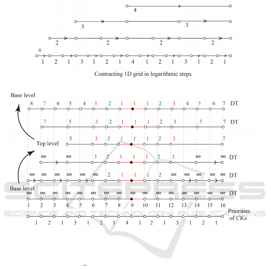
Figure 1: Edge contractions in the logarithmic way.
Figure 2: Computing of the DT in 1D grid.
follows:
D(v
i
) = min{D(v
i
), D(v
j
) +
(
1 i f T = 1
T
M
i f T ̸= 1
}
(6)
where
v
j
∈ N (v
i
), T = |Idx(v
i
) − Idx(v
j
)| (7)
An example of computing the DT in a 2D binary im-
age is shown in Fig. 3.
3 DEFINING THE DT IN A
COMBINATORIAL MAP
The distance transform [1] computes for every
pixel/voxel of an image/object how far it is from the
closest obstacle, or boundary, or background. Differ-
ent metrics can be used. In a topological data struc-
ture like a graph, a combinatorial map (Lienhardt,
1991), or a generalized map (Sansone et al., 2016)
often the shortest path between the obstacle/boundary
and a given point is used.
Let (D, α, σ) denote a two-dimensional combina-
torial map (2map). There are two versions of distance
transform on a 2map. One considers the edges α
∗
(d)
as a unit and counts the number of edges to follow
as the distance. This corresponds to the distance in
graphs. The alternative considers the darts d ∈ D as a
unit and the following neighbors for propagating dis-
tances:
Γ
2map
(d) = {α(d), σ(d), σ
−1
(d)} (8)
In the combinatorial map, each edge is replaced by
two darts. Therefore, computing the DT for darts pro-
vides double resolution for the resulting distance map.
Moreover, for every dimension 1, ..., n we receive one
distance, the distance through the highest dimension
n, and the (larger) geodesic distance along the bound-
ing i − cell, 0 < i < n. This characterizes more of a
ICPRAM 2023 - 12th International Conference on Pattern Recognition Applications and Methods
118

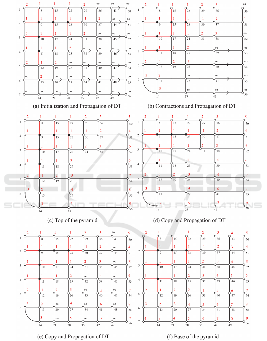
Figure 3: Computing of the DT in 2D grid.
Distance Transform in Parallel Logarithmic Complexity
119

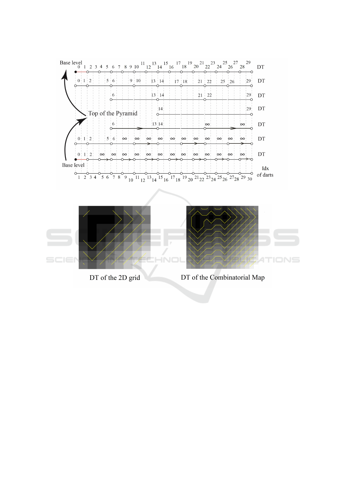
(a) Computing of the DT in 1D combinatorial map.
(b) DT in the 2D grid and in the CM of Fig. 3.
Figure 4: Computing the DT in combinatorial map.
shape than just the highest dimension. In addition, it
is a sort of map-edit-distance (Combier et al., 2013) in
analogy to the graph edit distance (Gao et al., 2010).
3.1 Logarithmic DT in a 1D
Combinatorial Map
To compute the DT in the CM, a similar algorithm to
Alg. 1 can be used but with two modifications. First,
the unique indices are defined for darts instead of ver-
tices. Second, in each step, we propagate distances by
α- and σ-propagation. The α-propagation of the DT
is performed as follows:
D(d
i
) = min{D(d
i
), D(α(d
i
)) + |Idx(d
i
) − Idx(α(d
i
))| }
(9)
Note that, during the contraction of the e = (d, α(d)),
the Idx(σ(d)) of the contracted dart is updated after
each contraction as follows:
Idx(σ(d)) = Idx(α(d)) (10)
The σ-propagation is performed as follows:
D(d
i
) = min{D(d
i
), D(σ(d
i
)) + 1, D(σ
−1
(d
i
)) + 1}
(11)
Fig. 4a shows an example of computing the DT in
1D CM. In constructing the pyramid in the bottom-
up procedure, first, the α-propagation and then the σ-
propagation are performed. In contrast, in the top-
down procedure, they are performed the other way
around. The steps of the algorithm are shown in
Alg. 2 and Fig. 4b displays the finer resolution of the
DT in comparison with the DT over 2D grid.
ICPRAM 2023 - 12th International Conference on Pattern Recognition Applications and Methods
120

Table 1: Execution (ms) of proposed Logarithmic DT, MeijsterGPU and FastGPU.
Image-size Mit. Log DT MRI Log DT Ran. Log DT Ran. MeijsterGPU Ran. FastGPU
256×256 0.0953 0.1209 0.0645 3.8524 1.7844
512×512 0.410 0.7310 0.3152 14.2005 4.2309
1024×1024 2.6308 5.1501 0.9364 25.8475 12.4668
2048×2048 4.1088 8.9506 1.8577 110.7817 44.9560
Figure 5: The proposed logarithmic DT over different images.
Algorithm 2: Computing DT in the 1D Combinatorial Map.
Input: CM = (D, α, σ)
Initialization: DT = ∞, ∀d ∈ D
3: DT (σ
∗
(d)) = 0, ∀d ∈ E
1
α- and σ-propagation to adjacent neighbors
Selecting the CKs (Bottom-up traversing)
6: While (DT = ∞ in the current level)
Contracting the edges with two unknown DT
α- and σ-propagation to adjacent neighbors
9: end (Top of the Pyramid)
For ( j = L downto 1) (Top-down traversing)
Imitate the DT from L → L − 1
12: σ- and α-propagation to adjacent neighbors
end
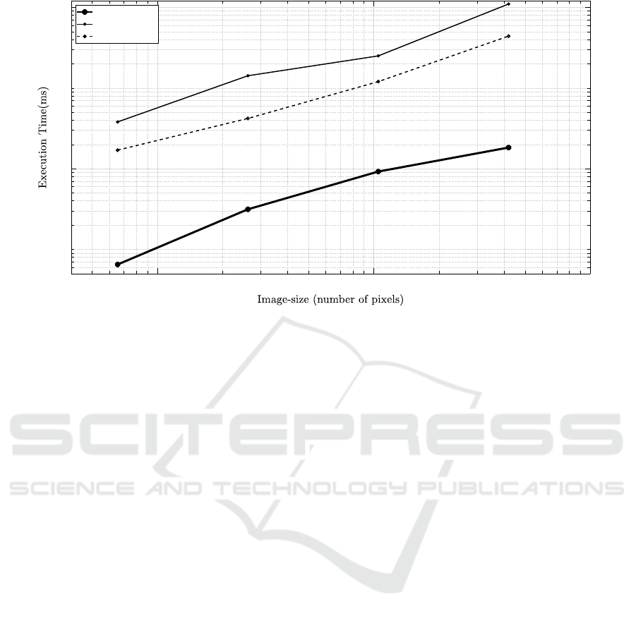
4 COMPARISONS AND RESULTS
To highlight the advantages of the proposed logarith-
mic algorithm, we compare the execution times with
two CUDA-based Implementations: MeijsterGPU
and FastGPU in (de Assis Zampirolli and Filipe,
2017). Simulations use MATLAB software employ-
ing CPU with AMD Ryzen 7 2700X, 3.7GHz, and
NVIDIA GeForce GTX 2080 TI that run over three
different categories of images: Random, Mitochon-
dria, and MRI. Table. 1 displays the outcome of the
implementations. The first column shows the im-
age size. The next three columns show the execu-
tion times (ms) of the proposed logarithmic DT (Log
DT) in the three different classes of images. The last
two columns show the execution time by the other two
methods. Fig. 5 compares the results of the logarith-
mic algorithm between the different classes. Since
the Random images contain smaller foreground ob-
jects than the other classes, they are executed faster.
In Fig. 6 the logarithmic method is compared to Mei-
jsterGPU and FastGPU methods. The logarithmic DT
is not only significantly faster than the other ones
but also has much higher performance dealing with
larger images. Note that all operations and processes
in the proposed algorithms are local and independent.
Therefore, each available thread of the GPU in the
shared memory is dedicated to each local process.
The bottleneck of the algorithms is the capacity of
the shared memory. Therefore, having sufficient inde-
pendent processing elements the algorithms are fully
parallel with logarithmic complexity.
Distance Transform in Parallel Logarithmic Complexity
121

10
5
10
6
10
7
10
0
10
2
Logarithmic DT
MeijsterGPU
FastGPU
Figure 6: Comparison of the proposed algorithm with MeijsterGPU and FastGPU (de Assis Zampirolli and Filipe, 2017).
5 CONCLUSION
Distance transform (DT) computes how far inside a
shape a point is located. In this paper, we study how
the distances can be calculated in a discrete domain
like a pixel grid and in combinatorial maps. Using the
irregular pyramid we proposed a new algorithm that
computes the DT in the logarithmic parallel complex-
ity. Moreover, by defining the DT over the combina-
torial maps, the smoother DT is calculated with dou-
ble precision. Using the dart ordering, we proposed
the logarithmic algorithm for computing the 1D com-
binatorial maps. However, the algorithm can be ex-
tended to higher n-dimensions. Finally, the practical
results show that the algorithm with parallel logarith-
mic complexity notably decreases the execution time
and makes it beneficial in particular for large images.
ACKNOWLEDGEMENTS
We acknowledge the Paul Scherrer Institut, Villi-
gen, Switzerland for the provision of beamtime at
the TOMCAT beamline of the Swiss Light Source
and would like to thank Dr. Goran Lovric for his
assistance. This work was supported by the Vi-
enna Science and Technology Fund (WWTF), project
LS19-013, and by the Austrian Science Fund (FWF),
projects M2245 and P30275.
REFERENCES
Banaeyan, M., Batavia, D., and Kropatsch, W. G. (2022).
Removing redundancies in binary images. In Interna-
tional Conference on Intelligent Systems and Patterns
Recognition (ISPR), Hammamet, Tunisia, March 24-
25, 2022, page 221–233. Springer.
Banaeyan, M. and Kropatsch, W. G. (2021). Pyrami-
dal connected component labeling by irregular graph
pyramid. In 5th International Conference on Pattern
Recognition and Image Analysis (IPRIA), pages 1–5.
Banaeyan, M. and Kropatsch, W. G. (2022a). Fast La-
beled Spanning Tree in Binary Irregular Graph Pyra-
mids. Journal of Engineering Research and Sciences,
1(10):69–78.
Banaeyan, M. and Kropatsch, W. G. (2022b). Par-
allel O(log(n)) computation of the adjacency of
connected components. In International Confer-
ence on Pattern Recognition and Artificial Intelli-
gence (ICPRAI), Paris, France, June 1-3, 2022, page
102–113. Springer.
Brun, L. and Kropatsch, W. (2003). Combinatorial pyra-
mids. In Proceedings of International Conference on
Image Processing, volume 2, pages II–33. IEEE.
Brun, L. and Kropatsch, W. G. (2012). Hierarchical graph
encodings. In L
´
ezoray, O. and Grady, L., editors,
Image Processing and Analysis with Graphs: Theory
and Practice, pages 305–349. CRC Press.
Brunet, D. and Sills, D. (2017). A generalized distance
transform: Theory and applications to weather analy-
sis and forecasting. IEEE Transactions on Geoscience
and Remote Sensing, 55(3):1752–1764.
Combier, C., Damiand, G., and Solnon, C. (2013). Map
edit distance vs. graph edit distance for matching im-
ages. In International Workshop on Graph-Based
ICPRAM 2023 - 12th International Conference on Pattern Recognition Applications and Methods
122

Representations in Pattern Recognition, pages 152–
161. Springer.
de Assis Zampirolli, F. and Filipe, L. (2017). A fast cuda-
based implementation for the euclidean distance trans-
form. In 2017 International Conference on High Per-
formance Computing Simulation (HPCS), pages 815–
818.
Fabbri, R., Costa, L. D. F., Torelli, J. C., and Bruno,
O. M. (2008). 2d euclidean distance transform algo-
rithms: A comparative survey. ACM Computing Sur-
veys (CSUR), 40(1):1–44.
Gao, X., Xiao, B., Tao, D., and Li, X. (2010). A survey of
graph edit distance. Pattern Analysis and applications,
13(1):113–129.
Hill, B. and Baldock, R. A. (2015). Constrained distance
transforms for spatial atlas registration. BMC bioin-
formatics, 16(1):1–10.
Kassis, M. and El-Sana, J. (2019). Learning free line detec-
tion in manuscripts using distance transform graph. In
2019 International Conference on Document Analysis
and Recognition (ICDAR), pages 222–227.
Kropatsch, W. G. (1995). Building irregular pyramids by
dual graph contraction. IEE-Proc. Vision, Image and
Signal Processing, Vol. 142(No. 6):pp. 366–374.
Lienhardt, P. (1991). Topological models for boundary rep-
resentation: a comparison with n-dimensional gener-
alized maps. Computer-aided design, 23(1):59–82.
Lindblad, J. and Sladoje, N. (2014). Linear time distances
between fuzzy sets with applications to pattern match-
ing and classification. IEEE Transactions on Image
Processing, 23(1):126–136.
Niblack, C., Gibbons, P. B., and Capson, D. W. (1992).
Generating skeletons and centerlines from the dis-
tance transform. CVGIP: Graphical Models and Im-
age Processing, 54(5):420–437.
Nilsson, O. and S
¨
oderstr
¨
om, A. (2007). Euclidian distance
transform algorithms: A comparative study.
Prakash, S., Jayaraman, U., and Gupta, P. (2008). Ear lo-
calization from side face images using distance trans-
form and template matching. In 2008 First Workshops
on Image Processing Theory, Tools and Applications,
pages 1–8. IEEE.
Rosenfeld, A. and Pfaltz, J. L. (1966). Sequential operations
in digital picture processing. Association for Comput-
ing Machinery, 13(4):471–494.
Sansone, C., Pucher, D., Artner, N. M., Kropatsch, W. G.,
Saggese, A., and Vento, M. (2016). Shape normaliz-
ing and tracking dancing worms. In Joint IAPR Inter-
national Workshops on Statistical Techniques in Pat-
tern Recognition (SPR) and Structural and Syntactic
Pattern Recognition (SSPR), pages 390–400.
Sobreira, H., Costa, C. M., Sousa, I., Rocha, L., Lima,
J., Farias, P., Costa, P., and Moreira, A. P. (2019).
Map-matching algorithms for robot self-localization:
a comparison between perfect match, iterative closest
point and normal distributions transform. Journal of
Intelligent & Robotic Systems, 93(3):533–546.
Distance Transform in Parallel Logarithmic Complexity
123