Football360: Introducing a New Dataset for Camera Calibration in

Sports Domain

Igor J

ano

and Vanda Bene

sov

Faculty of Informatics and Information Technologies, Slovak Technical University in Bratislava, Slovakia

Keywords:

Dataset, Radial Distortion, Camera Calibration, Sports, Football, Evaluation.

Abstract:

In many computer vision domains, the input images must conform with the pinhole camera model, where

straight lines in the real world are projected as straight lines in the image. Many existing camera calibra-

tion or distortion compensation methods have been developed using either ImageNet or other generic com-

puter vision datasets, but they are difﬁcult to compare and evaluate when applied to a speciﬁc sports domain.

We present a new dataset, explicitly designed for the task of radial distortion correction, consisting of high-

resolution panoramas of football arenas. From these panoramas, we produce a large number of cropped

images distorted using known radial distortion parameters. We also present extensible open-source software

to reproducibly export sets of training images conforming to the chosen radial distortion model. We evaluate

a chosen radial distortion correction method on the proposed dataset. All data and software can be found at

https://vgg.ﬁit.stuba.sk/football360.

1 INTRODUCTION

The sports domain has seen a boom in the use of com-

puter vision systems and tools. Many are used at the

amateur and top level for player tracking, collection

of statistical data, or as referee assistance. For precise

operation, they rely on some kind of camera calibra-

tion process that deals with radial distortion, which is

present in images captured by cameras with sophisti-

cated lens systems.

In the past, camera calibration was performed in

laboratory conditions using special calibration pat-

terns. In recent years, many methods based on deep

learning have appeared that are capable of estimat-

ing the radial distortion parameters from just a single

frame. However, these methods were often trained

on data originating from large popular datasets such

as ImageNet (Russakovsky et al., 2015), or SUN360

(Xiao et al., 2012), which are either not related to

sports or contain very few sports images. Strong vis-

ible lines are a typical feature of man-made objects.

In some methods, (Rong et al., 2017) only speciﬁc

subsets of data containing such strong lines were se-

lected for training. Many kinds of sports are played on

ﬁelds and courts marked with very distinctive lines.

However, these lines might not always be visible. Es-

pecially in football, the game is usually broadcasted

https://orcid.org/0000-0003-4783-6756

https://orcid.org/0000-0001-6929-9694

from a great distance, and only a small fraction of the

playﬁeld is visible at any given time. Bad weather or

football pitch condition can make the job of detect-

ing the ﬁeld lines even more challenging (Figure 1).

The scarcity of strong lines in sports images makes

it difﬁcult to evaluate and compare the effectivness of

general distortion correction methods when applied in

sports.

In this paper, we propose a new dataset of foot-

ball panorama images, a set of convenient exports of

images with known radial distortion parameters, and

an evaluation of a baseline radial distortion correction

method on the proposed dataset. We also propose a

set of tools that make it possible to apply the same

export- and evaluation- process on any other collec-

tion of panorama images, with the hope of aiding the

development of new and better radial distortion cor-

rection methods in the future.

The main contributions of this paper are:

• Collection of 268 high Resolution Panoramas -

captured from numerous positions all-around sev-

eral football arenas, capturing diverse lighting and

weather conditions (Section 3.1).

• Convenient Exports - offering training and valida-

tion data for convenient evaluation of radial dis-

tortion compensation methods (Section 3.3).

• Baseline Evaluation - of a selected method for ra-

dial distortion compensation (Section 4) on the

Jánoš, I. and Benešová, V.

Football360: Introducing a New Dataset for Camera Calibration in Sports Domain.

DOI: 10.5220/0011681200003417

In Proceedings of the 18th International Joint Conference on Computer Vision, Imaging and Computer Graphics Theory and Applications (VISIGRAPP 2023) - Volume 4: VISAPP, pages

301-308

ISBN: 978-989-758-634-7; ISSN: 2184-4321

 2023 by SCITEPRESS – Science and Technology Publications, Lda. Under CC license (CC BY-NC-ND 4.0)

301

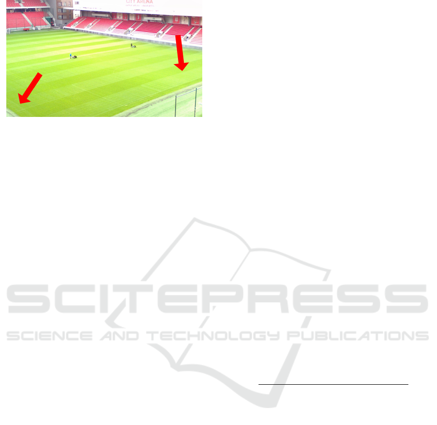
Figure 1: Image with very subtle pincushion distortion. The

football ﬁeld lines are very difﬁcult to spot.

proposed dataset.

• Exporting Tool - software with source code capa-

ble of producing training and evaluation data con-

forming to selected radial distortion model (Sec-

tion 3.4).

2 RELATED WORK

2.1 Related Datasets

Currently, there are several publicly available datasets

related to the sports domain. The Sports-1M dataset

presented by Karpathy et al. (Karpathy et al., 2014)

classiﬁes 1 million YouTube videos into 487 classes.

Datasets presented by Giancola et. al (Giancola et al.,

2018), Zanganeh et. al (Zanganeh et al., 2022), and

Jiang et. al (Jiang et al., 2020) help in signiﬁcant

events detection and football analysis. In (Zanganeh

et al., 2022) 33 football videos in a total time of 2508

minutes are annotated in 10 categories. These in-

clude the presence of the goal, free kick, yellow card,

red card, and others. Kazemi et. al (Kazemi et al.,

2013) have presented a multiview annotated dataset

for player pose estimation. The Soccer Video and

Player Position Dataset presented by Pettersen et. al

(Pettersen et al., 2014) contains images stitched from

three cameras spanning the entire football ﬁeld. And,

ﬁnally, the recent DeepSportradar-v1 (Van Zandycke

et al., 2022) introduces a set of tools, tasks, and data

for game analysis, court registration, and camera cal-

ibration in the basketball domain.

To the best of our knowledge, our proposed

dataset is the ﬁrst public sports domain dataset ded-

icated speciﬁcally to the task of radial distortion cor-

rection.

2.2 Camera Model

We assume a perspective projection camera model

with square pixels and a principal point located at the

center of the image sensor, as described in (Klette

et al., 1998). The perspective projection projects a

3D point p

= (X,Y,Z) into a 2D point on a plane

located at Z = 1 as normalized image coordinates

p = (x,y) = (X/Z,Y /Z). Scaling the normalized im-

age coordinates by the focal length f yields the result-

ing image pixel coordinates p

= (u, v) = ( f x, f y), rel-

ative to the image sensor center. This camera model is

referred to as a pinhole model. An important property

of the pinhole model is that it projects straight lines in

the real world into straight lines in observed images.

2.3 Radial Distortion Models

The distortion model is a mathematical relationship

that allows conversion between the observed distorted

image coordinates x = (x

) and the ideal pinhole

coordinates p = (x

). The polynomial model (Du-

ane, 1971) says that coordinates in the observed im-

ages are displaced away from or toward the image

center by an amount proportional to their radial dis-

tance. There is

x = (1 +k

∥

+ k

∥

+ k

∥

+ ···)p (1)

where k

,...are called the radial distortion pa-

rameters (or coefﬁcients).

The division model introduced by Fitzgibbon

(Fitzgibbon, 2001) is written as

p =

(1 + λ

∥

+ λ

∥

+ λ

∥

+ ···)

x (2)

where λ

,λ

,··· are coefﬁcients of the model.

The level of precision you can achieve by using any

one of these models is determined by the number of

coefﬁcients you wish to use. For many applications,

using just one coefﬁcient might be enough, however,

higher-order coefﬁcients might be necessary to model

complex distortion effects. The single-parameter di-

vision model is generally easier to work with and

also has the nice property of mapping straight lines

into circular arcs. Several methods tried to exploit

this and tried to estimate the distortion coefﬁcient by

ﬁtting circles into distinctive distorted lines in the

image (Bukhari and Dailey, 2013), or by detecting

distorted lines in a modiﬁed Hough space (Alem

an-

Flores et al., 2014). The likelihood of success of these

methods is depending on how well can they identify

the distorted lines in the image. In football, however,

these lines might be just too difﬁcult to spot, or not

VISAPP 2023 - 18th International Conference on Computer Vision Theory and Applications

302

visible at all (Figure 1). That is one of the reasons for

exploring learning-based methods of distortion cor-

rection.

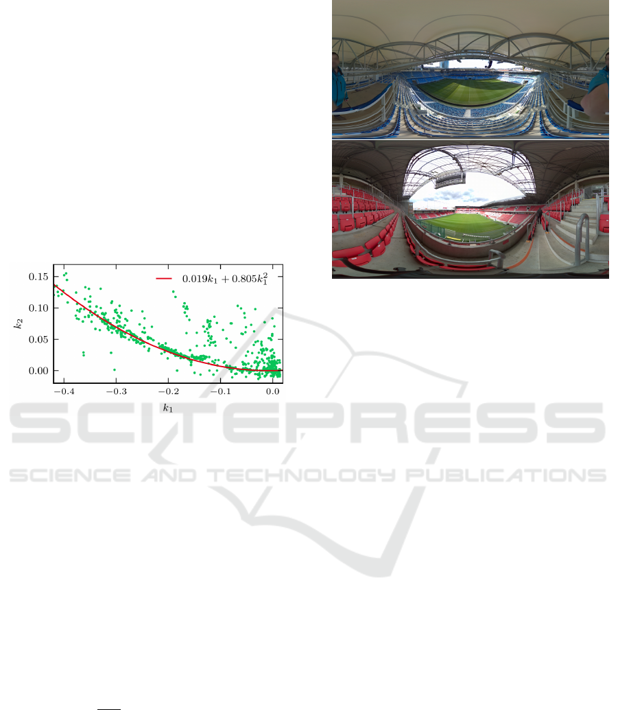
2.4 Distortion of Real Cameras

Lopez et al. (Lopez et al., 2019) have analyzed the

properties of real-world cameras. In their work they

have used Structure from Motion (SfM) with self-

calibration to estimate the distortion coefﬁcients on

a collection of 1000 street-level images captured with

more than 300 cameras (Figure 2). By ﬁtting a second

degree polynomial, they have obtained a model of the

observed distribution as:

= 0.019k

+ 0.805k

(3)

Figure 2: Distribution of the k

coefﬁcients recovered by

Lopez et al. (Lopez et al., 2019) from images captured by

more than 300 real-world cameras.

2.5 Metrics

When evaluating the accuracy of radial distortion cor-

rection, it feels natural to use L

, or L

distance be-

tween the ground truth and approximated coefﬁcients.

However, different groups of coefﬁcients may yield

similar levels of the distortion effect, which makes

distance metrics suboptimal for accuracy evaluations.

Also, it is not possible to compare the performance of

methods built using different distortion models. Liao

et. al (Liao et al., 2021) have proposed a new mean

distortion level deviation metric (MDLD),

MDLD =

W H

∑

i=1

∑

j=1

∥

d(i, j) − d(i, j)∥ (4)

where W and H are the width and height of the

image, and

d(i, j) is the distortion yielded by the ap-

proximated coefﬁcients of the given pixel, and d(i, j)

is the ground truth distortion. This metric is indepen-

dent of the chosen radial distortion model.

Additionally, we will also be using the structural

similarity index (SSIM), and peak signal-noise ratio

Figure 3: Example panorama images.

(PSNR) metrics (Hore and Ziou, 2010) to compare the

undistorted images using ground truth and estimated

coefﬁcients.

3 NEW DATASET

3.1 Panoramas

To capture our panoramas, we have used the commer-

cial Panono panoramic camera. The Panono camera

is equipped with 36 ﬁxed-focus cameras with 3.26

mm focal length distributed evenly over the cam-

era’s spherical surface. When capturing a panorama,

all of the cameras capture their part of the scenery

simultaneously. The Panono company provides an

automated cloud service to stitch the 36 captured

images into a single high-resolution equirectangular

panorama (16384 × 8192 pixels).

We have obtained 268 panorama images (Figure

3) from several football arenas. In each stadium, we

captured more than 50 panorama images from multi-

ple positions on multiple levels in the arena’s tribune

including broadcast camera platforms, each image of-

fering a unique view of the playﬁeld. The images con-

tained challenging lighting conditions, bad weather,

high contrast situations, football pitch maintenance

situations, and a regular football match with players

and referees to account for many possible situations

that may happen.

Football360: Introducing a New Dataset for Camera Calibration in Sports Domain

303

3.2 From Panoramas to Cropped

Images

From each of the panoramas, we have created a high

number of images by pointing an imaginary camera

standing in the center of the panorama in random di-

rections, and adjusting the zoom level randomly. The

resulting images would conform to the pinhole cam-

era model and would preserve straight lines from the

real world as straight lines in the image. Next, we in-

duced the radial distortion deﬁned by randomly sam-

pled distortion parameters, that become the ground

truth labels for our ﬁnal data (Figure 4). Later on a

deep neural network will try to learn to approximate

these distortion parameters.

When inducing barrel kind of distortion, the dis-

torted image might need to contain information from

outside the original undistorted image, which would

result in a typical rounded black frame (Figure 5).

Using a full panorama as a source, and integrating

the distortion computation directly within the map-

ping from panoramas to ﬁnal images helps to avoid

this problem.

We have decided to use two-parameter polyno-

mial model when inducing distortion, and we have

modeled the distribution of our sampled k

coefﬁ-

cients (Figure 6) as gaussian noise added to the man-

ifold (Equation 3) discovered by Lopez (Lopez et al.,

2019). We can divide real-world lenses into two cate-

gories - regular, and wide-angle. Regular lenses usu-

ally induce only a small amount of distortion (k

close to zero), but we can see in the Figure 2, that

even for values of k

close to zero, there is a signiﬁ-

cant distribution of non-zero k

coefﬁcients, and that

single-parameter distortion models, both polynomial

and division, are not sufﬁcient enough to correct such

distortion. Wide-angle lenses (k

is smaller than zero)

induce much stronger distortion effect, which is dom-

inated by the k

coefﬁcient.

3.3 Convenient Exports

We have split the 268 panoramas into two subsets

in 90%/10% ratio, and from these subsets we have

decided to create three sets of exported images for

training, and one set for validation. We believed it

might be useful to see what impact would the size of

the training data have on the ﬁnal performance of the

distortion compensation methods, as well as on the

progress of training, and speed of convergence.

We have decided to render the images in 1920 ×

1080 pixels resolution with the 16 : 9 image aspect

ratio, which is standard for TV broadcast today. And

then resize them down to 448 × 448 pixels resolution.

Table 1: Properties of the export sets.

Set Purpose Images Size

A Training 30,000 10.5 GB

B Training 100,000 35.2 GB

C Training 300,000 105.5 GB

V Validation 10,000 3.5 GB

Table 2: Distribution of the camera parameters used to gen-

erate the synthesized data set.

Parameter Distribution Values

Pan Uniform [−40

◦

;40

◦

]

Tilt Uniform [−25

◦

;−2

◦

]

Roll Uniform [−2

◦

]

Field of view Uniform [10

◦

;50

◦

]

Uniform [−0.45;0.12]

noise of k

Normal µ = 0.0,σ = 0.02

Many publicly available pre-trained feature extractor

models operate in native 224 × 224 pixels resolution,

which can be easily achieved by using proper input

transformation during training. Having the conve-

nient exports in higher resolution also offers the pos-

sibility to experiment with custom models that might

beneﬁt from ﬁner image details.

Finally, we have saved the images as PNG (8-bits

per each color channel) and stored them in a single

HDF5 ﬁle, which is very convenient to work with.

The properties of the ﬁnal export sets are summa-

rized in table 1.

The properties of the distributions of view pa-

rameters and induced radial distortion parameters are

summarized in table 2.

3.4 Exporting Tool

We have used the C++ programming language,

OpenGL library, and GLSL shaders to develop a com-

mand line exporting tool. The exporting tool can

be conﬁgured using JSON ﬁles to reproducibly gen-

erate export sets. The exporting process is opti-

mized to run well on modern GPUs, and is capa-

ble of producing a dataset containing 300,000 im-

ages in just a few hours. Please, refer to the GitHub

project (https://github.com/IgorJanos/stuFootball360)

for more information on how to customize the conﬁg-

uration ﬁles.

4 EVALUATION

We have decided to choose the work of Lopez et. al.

(Lopez et al., 2019) as the baseline method. Com-

VISAPP 2023 - 18th International Conference on Computer Vision Theory and Applications

304

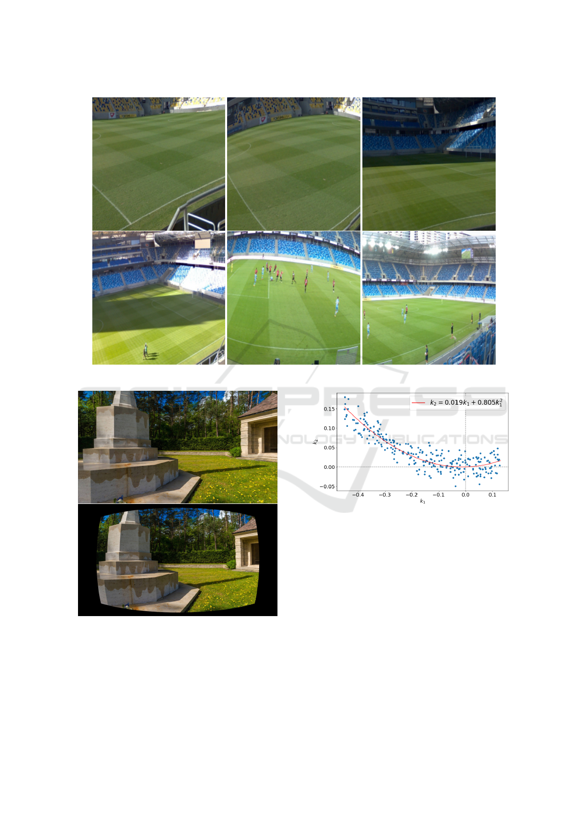
Figure 4: Example cropped and distorted images.

Figure 5: An image conforming to the pinhole camera

model (top), and a black frame around the artiﬁcially in-

duced barrel distortion (bottom).

pared to the original method, we have made only a

minor modiﬁcation and removed the regressor heads

estimating pan, tilt, and ﬁeld of view, which are not

relevant to our task. We have decided to use a 2-

Figure 6: Distribution of the k

coefﬁcients sampled

from the distribution summarized in table 2.

parameter polynomial model as described in section

2.3. Our neural network consists of a backbone fea-

ture extractor, and a single regressor to approximate

the k

coefﬁcient. The regressor head consists of a

single hidden dense layer containing 256 units with

BatchNorm, and ReLU activation, followed by a sin-

gle output unit yielding the estimated k

coefﬁcient.

From the estimated k

coefﬁcient, we will compute

the value of k

using the equation 3.

We have selected three contemporary con-

volutional architectures - DenseNet-161 (Huang

et al., 2017), ResNet-152 (He et al., 2016), and

EfﬁcientNet-B5 (Tan and Le, 2019) as our backbone

feature extractors, and studied their behavior during

the training on all export sets. All feature extractors

Football360: Introducing a New Dataset for Camera Calibration in Sports Domain

305

were pretrained on the ImageNet dataset.

To be able to evaluate the progress of training

on datasets of different sizes, we have decided to ﬁx

the length of a single epoch to 1000 iterations. This

means, that the model will be trained on the same total

number of training images, looping over the smaller

datasets more often than over the larger ones. We have

set the number of epochs to 150, and batch size to 64.

This gives us 9.6 million training images for the entire

training.

We have used Adam optimizer (Kingma and Ba,

2014) with learning rate equal to 0.0001, and applied

exponential decay of 0.985 after each epoch (after

1000 iterations). We have observed no signiﬁcant

difference between training with L

loss and Huber

loss and decided to train with L

loss. On a system

equipped with two RTX3090 GPUs, the training and

evaluation of a single set took about 15 hours to ﬁnish.

All nine sets were processed in about six days.

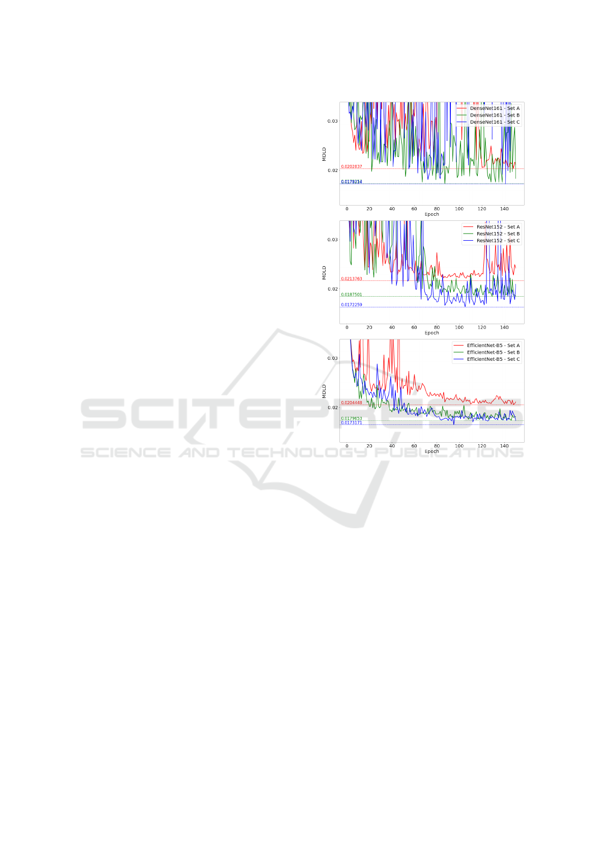
4.1 Training

During the training process, we observed that all

backbone models experienced phases of highly in-

consistent accuracy on the validation data (Figure 7).

Among the chosen backbones, the EfﬁcientNet model

performed the most consistently, and after the ini-

tial 50 epochs, the accuracy stabilized and improved

steadily over time. One can see, that there is an ex-

pected signiﬁcant accuracy gap between the small-

est set A and the larger sets B and C. The difference

between the B and C sets is rather small, especially

with the EfﬁcientNet model. It is also interesting, that

when training on larger sets the accuracy will surpass

the best results achieved by training on set A in just

under 50 epochs on all backbone models. It is also in-

teresting, that the best accuracy was achieved some-

where around the epoch 100 on all backbone mod-

els. One can conclude, that an early stopping strategy

might have saved some computation time.

4.2 Results

We have analyzed the distribution of k

prediction er-

ror on all backbones (Figure 10). We have noticed,

that all backbones behaved similarly, and have felt

more conﬁdent estimating stronger distortion, where

the total distortion effect was dominated by the single

coefﬁcient. On the intervals of k

corresponding to

smaller distortion, the models were less certain. We

attribute this to the presence of an additional distor-

tion effect due to the noisy k

coefﬁcient, which the

model predicting only a single distortion coefﬁcient

was less likely to grasp.

Figure 7: The progress of training on DenseNet-161 (top),

ResNet-152 (middle), and EfﬁcientNet-B5 (bottom) back-

bones. The graph displays the value of MDLD calculated

on the validation set after each training epoch.

It is also important to note, that for images con-

taining only a very small amount of distortion an at-

tempt to correct it might even be harmful, because for

values close to 0 the variance of prediction error

seems to be the highest.

On models trained on the smallest training set A,

one can see an obvious bias problem on both extremes

of the k

range (Figure 9). We might conclude, that a

training set of 30,000 images might just be too small

for proper training of the baseline distortion correc-

tion method.

5 CONCLUSION

This paper introduces a new dataset to aid the devel-

opment and evaluation of methods for radial lens dis-

tortion correction. We provide a set of convenient ex-

ports for direct comparison of future methods. We

VISAPP 2023 - 18th International Conference on Computer Vision Theory and Applications

306

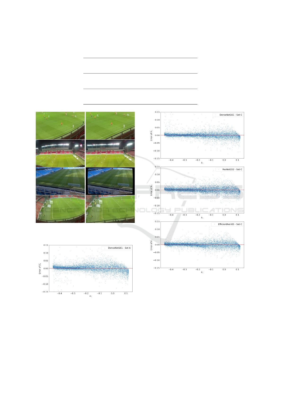
Table 3: Results of all evaluated metrics on the best-performing models.

Backbone Set SSIM ↑ PSNR ↑ MDLD ↓

DenseNet-161 A 0.829 22.323 dB 0.02028

B 0.847 22.906 dB 0.0180

C 0.850 23.085 dB 0.01782

ResNet-152 A 0.822 22.127 dB 0.02138

B 0.840 22.699 dB 0.01875

C 0.852 23.075 dB 0.01723

EfﬁcientNet-B5 A 0.828 22.274 dB 0.02044

B 0.846 22.789 dB 0.01797

C 0.850 22.976 dB 0.01732

Figure 8: Distorted images (left column), and corrected im-

ages using the estimated distortion coefﬁcients (right col-

umn).

Figure 9: Bias problem on the extremes of the k

range

when trained on the training set A.

also provide means for reproducing the dataset ex-

porting process for other domains just by changing

the source panorama images. And, we also provide

means for easy extension of the radial distortion mod-

els used.

Figure 10: The distribution of errors of the estimated

coefﬁcients over the range of k

on DenseNet-161 (top),

ResNet-152 (middle), and EfﬁcientNet-B5 (bottom) back-

bones.

In our experiments, we have evaluated a baseline

method with multiple contemporary feature extractor

models, and provided baseline results using metrics

that are independent of the radial distortion model

used.

Our future work will include the possible im-

provement of the baseline method in terms of speed

Football360: Introducing a New Dataset for Camera Calibration in Sports Domain

307

and accuracy. We will explore the possibility of train-

ing a model to predict the distortion coefﬁcients inde-

pendently. We will also focus on the task of estimat-

ing the camera pose with respect to the playﬁeld.

REFERENCES

Alem

an-Flores, M., Alvarez, L., Gomez, L., and Santana-

Cedr

es, D. (2014). Automatic lens distortion correc-

tion using one-parameter division models. Image Pro-

cessing On Line, 4:327–343.

Bukhari, F. and Dailey, M. N. (2013). Automatic radial

distortion estimation from a single image. Journal of

mathematical imaging and vision, 45(1):31–45.

Duane, C. B. (1971). Close-range camera calibration. Pho-

togramm. Eng, 37(8):855–866.

Fitzgibbon, A. W. (2001). Simultaneous linear estimation

of multiple view geometry and lens distortion. In Pro-

ceedings of the 2001 IEEE Computer Society Con-

ference on Computer Vision and Pattern Recognition.

CVPR 2001, volume 1, pages I–I. IEEE.

Giancola, S., Amine, M., Dghaily, T., and Ghanem, B.

(2018). Soccernet: A scalable dataset for action spot-

ting in soccer videos. In Proceedings of the IEEE

conference on computer vision and pattern recogni-

tion workshops, pages 1711–1721.

He, K., Zhang, X., Ren, S., and Sun, J. (2016). Deep resid-

ual learning for image recognition. In Proceedings of

the IEEE conference on computer vision and pattern

recognition, pages 770–778.

Hore, A. and Ziou, D. (2010). Image quality metrics: Psnr

vs. ssim, in ‘2010 20th international conference on

pattern recognition’. Istanbul: IEEE, pages 2366–

2369.

Huang, G., Liu, Z., Van Der Maaten, L., and Weinberger,

K. Q. (2017). Densely connected convolutional net-

works. In Proceedings of the IEEE conference on

computer vision and pattern recognition, pages 4700–

4708.

Jiang, Y., Cui, K., Chen, L., Wang, C., and Xu, C. (2020).

Soccerdb: A large-scale database for comprehensive

video understanding. In Proceedings of the 3rd Inter-

national Workshop on Multimedia Content Analysis in

Sports, pages 1–8.

Karpathy, A., Toderici, G., Shetty, S., Leung, T., Suk-

thankar, R., and Fei-Fei, L. (2014). Large-scale video

classiﬁcation with convolutional neural networks. In

Proceedings of the IEEE conference on Computer Vi-

sion and Pattern Recognition, pages 1725–1732.

Kazemi, V., Burenius, M., Azizpour, H., and Sullivan, J.

(2013). Multi-view body part recognition with ran-

dom forests. In 2013 24th British Machine Vision

Conference, BMVC 2013; Bristol; United Kingdom;

9 September 2013 through 13 September 2013. British

Machine Vision Association.

Kingma, D. P. and Ba, J. (2014). Adam: A

method for stochastic optimization. arXiv preprint

arXiv:1412.6980.

Klette, R., Koschan, A., and Schluns, K. (1998). Three-

dimensional data from images. Springer-Verlag Sin-

gapore Pte. Ltd., Singapore.

Liao, K., Lin, C., and Zhao, Y. (2021). A deep ordinal dis-

tortion estimation approach for distortion rectiﬁcation.

IEEE Transactions on Image Processing, 30:3362–

3375.

Lopez, M., Mari, R., Gargallo, P., Kuang, Y., Gonzalez-

Jimenez, J., and Haro, G. (2019). Deep single image

camera calibration with radial distortion. In Proceed-

ings of the IEEE/CVF Conference on Computer Vision

and Pattern Recognition, pages 11817–11825.

Pettersen, S. A., Johansen, D., Johansen, H., Berg-

Johansen, V., Gaddam, V. R., Mortensen, A.,

Langseth, R., Griwodz, C., Stensland, H. K., and

Halvorsen, P. (2014). Soccer video and player posi-

tion dataset. In Proceedings of the 5th ACM Multime-

dia Systems Conference, pages 18–23.

Rong, J., Huang, S., Shang, Z., and B, X. Y. (2017). Radial

lens distortion correction using convolutional neural

networks trained with synthesized images. Computer

Vision – ACCV 2016, pages 35–49.

Russakovsky, O., Deng, J., Su, H., Krause, J., Satheesh, S.,

Ma, S., Huang, Z., Karpathy, A., Khosla, A., Bern-

stein, M., et al. (2015). Imagenet large scale visual

recognition challenge. International journal of com-

puter vision, 115(3):211–252.

Tan, M. and Le, Q. (2019). Efﬁcientnet: Rethinking model

scaling for convolutional neural networks. In Interna-

tional conference on machine learning, pages 6105–

6114. PMLR.

Van Zandycke, G., Somers, V., Istasse, M., Don, C. D., and

Zambrano, D. (2022). Deepsportradar-v1: Computer

vision dataset for sports understanding with high qual-

ity annotations. In Proceedings of the 5th Interna-

tional ACM Workshop on Multimedia Content Analy-

sis in Sports, pages 1–8.

Xiao, J., Ehinger, K. A., Oliva, A., and Torralba, A. (2012).

Recognizing scene viewpoint using panoramic place

representation. Proceedings of the IEEE Computer

Society Conference on Computer Vision and Pattern

Recognition, pages 2695–2702.

Zanganeh, A., Jampour, M., and Layeghi, K. (2022). Iaufd:

A 100k images dataset for automatic football im-

age/video analysis. IET Image Processing.

VISAPP 2023 - 18th International Conference on Computer Vision Theory and Applications

308