Qualitative Spatial Representation and Reasoning About Fold Strata
Yuta Taniuchi and Kazuko Takahashi
School of Engineering, Kwansei Gakuin University, 1, Gakuen, Uegahara, Sanda, 669-1330, Japan
Keywords:
Qualitative Spatial Reasoning, Knowledge Representation, Logical Reasoning, Shape Information.
Abstract:
We propose a method of handling strata in qualitative spatial representation. We make a model for a typical
fold structure projected onto a two-dimensional plane extracted by a rectangle. It is expressed by a pair of
sequences of symbols that represents the strata configuration and the shape of the layers, respectively. We
define the validity required of the representation and show that the representation and the model have a one-to-
one relation. Moreover, we define operations on the representation, such as rotation and symmetric transitions,
and show that validity is preserved. We also show that global data can be constructed by connecting local data.
This method can provide a logical explanation of the processes involved in strata-generation prediction, which
in the field of structural geology have been examined manually to date, and find results that manual analysis
may overlook.
1 INTRODUCTION
Temporal changes in a landscape have a strong re-
lationship with the occurrence of natural disasters.
Thus, to predict future events, such as landslides,
earthquakes or river flooding, there is a need to elu-
cidate the formation processes of specific landscapes
and the causality of the changes involved. To con-
sider morphological changes, investigation of strata
is an essential component.
In structural-geology research (Kano and Murata,
1998), the shapes and structures of strata are analyzed
using data at various scales, from the micro level, such
as collected small sample data measured in tens of
centimeters, or slices thereof that can be observed by
microscopy, to the macro level at the out-crop scale of
several-hundred meters, or aerial photos of larger re-
gions. Regardless of scale, the entire shape of a stra-
tum is estimated by integrating local data collected
from multiple locations, since in a real landscape it
is rare for an entire stratum to be exposed. Since hu-
man error may affect this process. a method that can
overcome this shortcoming is required.
In this study, we propose a novel approach that
uses qualitative spatial reasoning (QSR), which is a
subfield of artificial intelligence. QSR represents spa-
tial entities symbolically without using concrete nu-
merical data, and enables reasoning on the represen-
tation (Cohn and Renz, 2008; Chen et al., 2013;
Ligozat, 2011; Sioutis and Wolter, 2021). Represen-
tation focuses on specific aspects or properties of an
object or the relation of objects, depending on the
user’s purpose, such as mereological relations, the rel-
ative positions or directions of objects, rough shapes,
and on on. Avoiding the need for precise values en-
ables a small computational burden, and declarative
representation suits human recognition. So far, lots
of works have been done depending on the focused
aspects of spatial data.
To apply QSR to the shapes of strata, there are
two primary requirements: one layer continues in one
direction if there is no fault, and the relations of inter-
layer connections remain unchanged even if a stratum
rotates or bends.
Although it is rather difficult to consider shape
in QSR, several researchers have proposed handling
the shape of an object by projecting it onto a two-
dimensional plane (Cohn, 1995; Falomir et al.,
2013; Galton and Meathrel, 1999; Kulik and Egen-
hofer, 2003; Kumokawa and Takahashi, 2008; Ley-
ton, 1988; Cabedo and Escrig, 2004; Cabedo et al.,
2010; Pich and Falomir, 2018; Tosue and Takahashi,
2019). In most of these studies, a set of primitives
was introduced and the shape of the object was rep-
resented by arranging these primitives in the order of
their occurrence when tracing the outline of the ob-
ject. This process indicates that the target is essen-
tially one-dimensional spatial data.
On the other hand, for our application, we have to
consider representation based on local data extracted
Taniuchi, Y. and Takahashi, K.
Qualitative Spatial Representation and Reasoning About Fold Strata.
DOI: 10.5220/0011677900003393
In Proceedings of the 15th International Conference on Agents and Artificial Intelligence (ICAART 2023) - Volume 2, pages 211-220
ISBN: 978-989-758-623-1; ISSN: 2184-433X
Copyright
c
 2023 by SCITEPRESS – Science and Technology Publications, Lda. Under CC license (CC BY-NC-ND 4.0)
211

from a stratum, since the entire data do not com-
prise a closed curve. Moreover, we have to represent
not only the shapes of layers that become regions of
a two-dimensional plane but also their interconnec-
tions. Therefore, we cannot apply existing methods.
In this study, we propose representation and rea-
soning for a fold as a relatively simple strata struc-
ture. First, we define a model for local fold data and
the language needed to describe it. Next, we define
the validity required of the representation, and show
that the model representation is valid and that a figure
can be drawn on a two-dimensional plane for the valid
representation. Moreover, we define operations on the
representation corresponding to rotation and symmet-
ric transitions, and show that validity is preserved. Fi-
nally, we discuss the interconnection of models that
have the same strata configurations. Our goal is to
derive spatial relations among multiple local data col-
lected in different places or at different times.
This study provides a mechanical treatment of
strata using symbolic representation that focuses on
their features. This approach can provide logical ex-
planations of processes that may be involved in fu-
ture morphological changes that manual analysis may
overlook.
This paper is organized as follows. In Section 2,
we identify our target fold and the model thereof .
In Section 3, we define a description language. In
Section 4, we provide an algorithm to generate a rep-
resentation for a model, and show that the represen-
tation and the model have a one-to-one relation. In
Section 5 we define operations on this representation.
In Section 6, we discuss reasoning using these opera-
tions. In Section 7, we compare our study with related
studies. Finally, in Section 8, we show our conclu-
sions and future works.
2 MODEL
We describe a typical form of fold strata such as that
shown in Figure 1(a). We assume that there is no
fault or hole, and that the curvature of all the lay-
ers is the same. We model a vertical cross section
of the fold projected onto a two-dimensional plane.
We derive the local data extracted from the global
data by a rectangle that satisfies the following con-
ditions [COND]. Based on these conditions, the fold
is divided into regions using multiple smooth con-
tinuous curves (called layer-borderlines). Pairs of
layer-borderlines do not intersect and there is no self-
intersection. We treat this figure as our model.
[COND]
1. All layers and any space (a region containing no
(a) fold form (b) model on a 2D plane
Figure 1: A model for a fold.
layer) in the global data appear to be connected
regions in the local data.
2. The end-points of each layer-borderline are not lo-
cated on a corner of the rectangle.
3. Each layer-borderline is a smooth curve with nei-
ther an extremum nor an inflection point.
For example, part of the fold shown in Figure 1(a)
is modeled as the figure in Figure 1(b). In the model,
the bottom-left point is regarded as the origin and the
inclination of the curve is determined to be either in-
creasing or decreasing.
We refer to the borderlines between layers as
layer-borderlines to discriminate them from the bor-
derline of the rectangle.
Note that since this is a qualitative model, we fo-
cus only on the side on which end-points of layer-
borderlines occur and the order of the locations, ig-
noring their precise positions. As for the shape of a
layer-borderline, we focus only on its inclination and
convexity, ignoring its precise shape. As a result, sev-
eral figures are regarded as the same model.
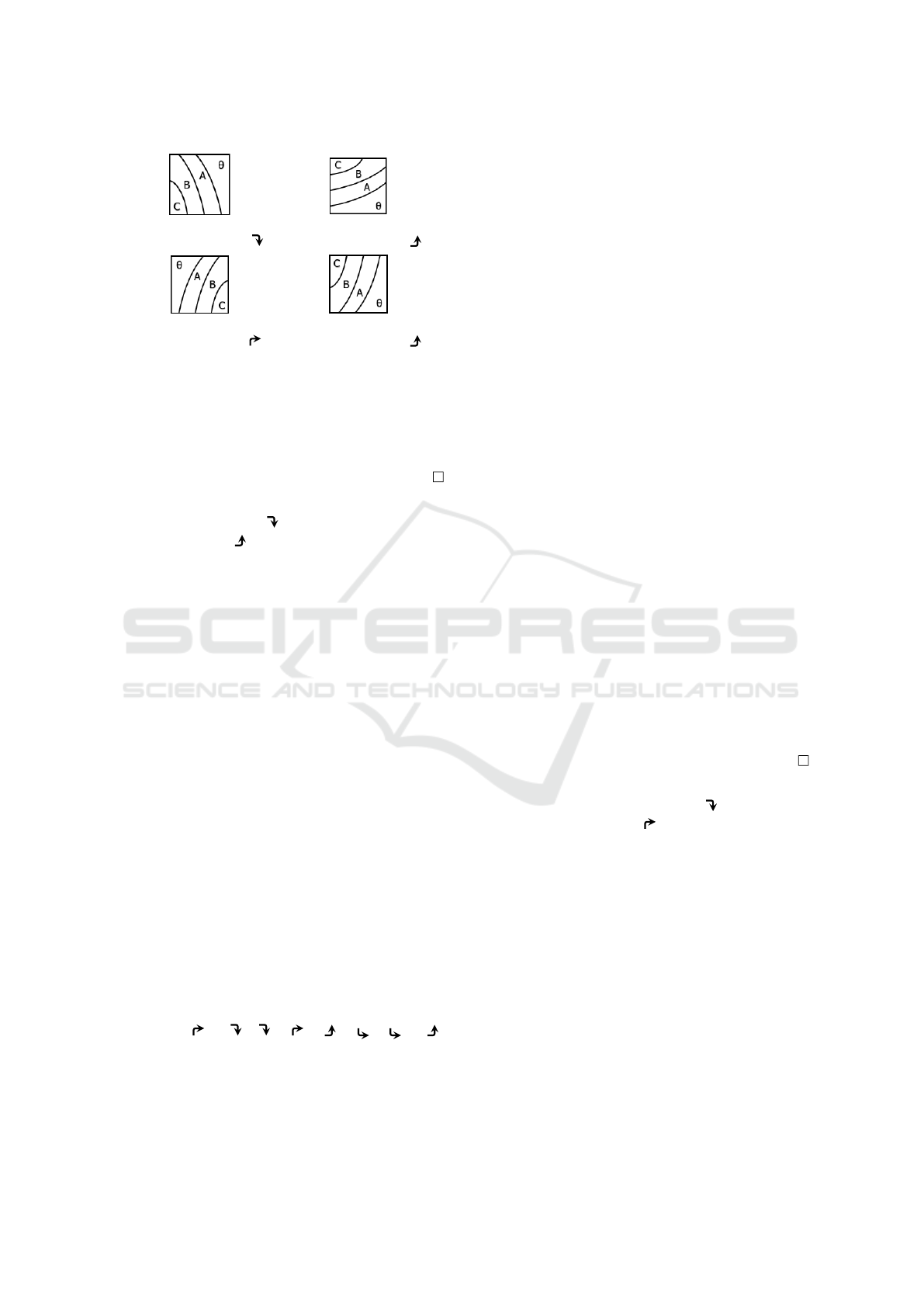
Example 1. In Figure 2, (b) is regarded as the same
model as (a), whereas (c) and (d) are not.
(a) (b)
(c) (d)
Figure 2: Models.
3 DESCRIPTION LANGUAGE
3.1 Language
We define two kinds of description languages Lang1
and Lang2 to represent the model for local data.
ICAART 2023 - 15th International Conference on Agents and Artificial Intelligence
212

Lang1 is used to describe the configuration of a
stratum. This is defined as Lang1 = {A
1
,...,A
n
} ∪
{θ} where A
1
,...,A
n
are the names of the layers and
θ denotes the outside of the stratum. A
1
,...,A
n
and θ
are called layer-symbols.
Lang2 is used to describe the shape of a layer-
borderline. This is defined as Lang2 = { , , , }
where , , and indicate convex upward and
increasing, convex upward and decreasing, convex
downward and increasing, and convex downward and
decreasing, respectively. , , and are called
shape-symbols. We also denote U p = { , },Dn =
{ , }.
Let σ = e
1
...e
k
be either a sequence of symbols
in Lang1 or that of those in Lang2. If σ is the null
sequence, then we denote it as ε. For each i (1 ≤ i ≤
k), we denote e
i
∈ σ. We also denote f irst(σ) = e
1
,
last(σ) = e
k
and σ
−1
= e
k
...e
1
for i ≥ 1.
Definition 1 (local data description, layer-sequence).
Local data description is defined as a pair (L,C),
where L and C are finite sequences that include sym-
bols in Lang1 and Lang2, respectively. L consists of
four segments in the form (σ
1
)(σ
2
)(σ
3
)(σ
4
) with aux-
iliary symbols ’(’ and ’)’. The sequence of symbols
without the auxiliary symbols ’(’ and ’)’ is called a
layer-sequence of L.
A layer-sequence is considered cyclic data, that is,
for a layer-sequence e
1
...e
k
, e
0
is considered e
k
, and
for all i (1 ≤ i ≤ k), e
i
...e
k
e
1
...e
i−1
are considered
the same data.
Definition 2 (sequence-of-transitions). For a local
data description (L,C), let I = e
1
,...,e
k
be a layer-
sequence of L, where k 6= 1. Then the sequence
c
1
...c
k
where for each i (1 ≤ i ≤ k), c
i
= e
i−1
/e
i
,
e
i
∈ σ
i
, σ
i
∈ {σ
1
,σ
2
,σ
3
,σ
4
} is said to be a sequence-
of-transitions of L. And we denote chgpt(c
i
,σ
i
).
Example 2. For L = (Aθ)()(ABC)(B), the layer-
sequence of L is I = AθABCB, the sequence-of-
transitions of L is B/A,A/θ,θ/A,A/B,B/C,C/B, and
chgpt(A/θ,σ
1
) and chgpt(θ/A, σ
3
) hold.
3.2 Validity
For the local data description (L,C) where L =
(σ
1
)(σ
2
)(σ
3
)(σ
4
), we introduce the term ‘inclination
of a layer-borderline’ that relates L and C.
Definition 3 (inclination of a layer-borderline). For
each pair of layer-symbols X and Y , for which
chgpt(X/Y,σ) and chgpt(Y /X, σ
0
) where σ 6= σ
0
hold, the inclination of a layer-borderline C
XY
is
defined depending on the pair of σ and σ
0
as follows:
• if (σ,σ
0
) is either (σ
1
,σ
2
),(σ
2
,σ
1
),(σ
3
,σ
4
) or
(σ
4
,σ
3
), then C
XY
= dn
• if (σ,σ
0
) is either (σ
1
,σ
4
),(σ
2
,σ
3
),(σ
3
,σ
2
) or
(σ
4
,σ
1
), then C
XY
= up
• otherwise C
XY
= any.
Definition 4 (validity). If the local data description
(L,C) satisfies the following conditions, then it is said
to be a valid representation.
Let L = (σ
1
)(σ
2
)(σ
3
)(σ
4
) and its layer-sequence
I = e
1
...e
k
.
v1 For any pair X and Y of layer-symbols if L in-
cludes chgpt(X/Y, σ), then it includes exactly one
chgpt(Y /X,σ
0
), where σ 6= σ
0
holds.
v2 I is X
n
θ or in the form of X
1
...X
n−1
X
n
X
n−1
...X
1
θ
where X
i
6= X
j
(1 ≤ i < j ≤ n).
v3 |C| = 1.
v4 • If for all C
XY
, C
XY
= up or any, then C ∈ U p.
• If for all C
XY
, C
XY
= dn or any, then C ∈ Dn.
• otherwise, C ∈ U p ∪ Dn.
From [v2], the following proposition holds.
Proposition 1. Let (L,C) be a valid representation
and I be a layer-sequence of L. Then I = I
−1
.
4 REPRESENTATION FOR A
MODEL
We provide a representation for a model. We show
that it is valid; and that conversely there exists a model
of a valid representation and we can draw a figure sat-
isfying [COND].
4.1 Representation for a Model
When a model M of local data is provided, starting
from the top-left of M, trace the borderline of M in a
clockwise manner to obtain a sequence of the layer-
symbols that are encountered, and place parenthe-
ses around each side of the rectangle. Then we set
L = (σ
t
)(σ
r
)(σ
b
)(σ
l
), where σ
t
,σ
r
,σ
b
and σ
l
are the
sequence of upper side, right side, lower side and left
side of the rectangle, respectively. We set C to cor-
respond to the shape of the layer-borderline. (Note
that the shape of all the layer-borderlines is the same.)
Then D = (L,C) is said to be a representation for M,
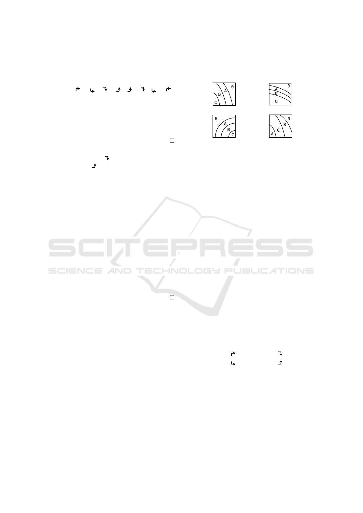
Example 3. The representation for the model shown
in Figure 3 is ( (Aθ)()(ABC)(B),
).
The sequence starts not from layer-symbol B, but
from A, although this may seem unnatural. If the
sequence were to start from B, the layer-symbol oc-
cupying the top-left corner would appear in both σ
t
Qualitative Spatial Representation and Reasoning About Fold Strata
213

Figure 3: Representation for a model.
and σ
l
. To avoid such a situation and to treat the
sequence cyclically, the sequence starts from A, the
layer-symbol that is encountered first on tracing.
Let (L,C) be a representation for the model M.
The sequence-of-transitions c
1
...c
k
of L shows the
order of occurrence of the end-points of each layer-
borderline on tracing the borderline of M. And for
each i (1 ≤ i ≤ k), chgpt(c
i
,σ
i
) indicates that the end-
point c
i
of a layer-borderline is on the side corre-
sponding to σ
i
.
4.2 Validity and Drawability
Theorem 1 (validity of the model). The representa-
tion for the model is valid.
Proof. For any pair X and Y of layer-symbols,
chgpt(X/Y,σ) and chgpt(Y /X, σ
0
) correspond to the
two end-points of the layer-borderline of X and Y .
From the first condition of [COND], each layer-
borderline of M does not intersect with itself or an-
other layer-borderline. It has exactly two end-points
on the borderlines, which are not on the same side of
M, in accordance with the third condition of [COND].
Therefore, σ 6= σ
0
. Thus, validity [v1] holds.
The length of each layer-sequence is even, since
each layer-borderline has exactly two end-points. Let
e
1
...e
2k
be the layer-sequence of L. If there is only
one layer-borderline, then the layer-sequence of L
is X θ where X is a layer-symbol. If there is more
than one layer-borderline, then let e
0
= e
2k
= θ, e
1
=
X
1
,...,e
k
= X
k
, where X
i
∈ Lang1 (1 ≤ i ≤ k). For
each i, j (0 ≤ i < j ≤ k − 1), if the end-points X
i
/X
i+1
and X
j
/X
j+1
occur in this order in L, then X
j+1
/X
j
and X
i+1
/X
i
occur in this order in L, since layer-
borderline pairs should not intersect. Moreover, if we
assume that X
i
= X
j
(i 6= j) holds, then the layer X
i
should appear more than twice in L, indicating that it
is a disconnected region; this contradicts the first con-
dition of [COND]. Therefore, X
i
6= X
j
. Thus, validity
[v2] holds.
Validity [v3] holds from the assumption of the
model. Therefore, C
XY
are defined uniquely and con-
sistently for all pairs of X and Y . Thus, validity [v4]
holds.
Theorem 2 (drawability of the representation). There
exists a model for the valid representation.
Proof. Let (L,C) be a valid representation and L =
(σ
1
)(σ
2
)(σ
3
)(σ
4
).
Let c
1
...c
2k
be a sequence-of-transitions of L,
since the lengths of sequence-of-transitions of L are
even from validity [v2]. We locate each c
i
∈ σ
i
(σ
i
∈ {σ
1
,σ
2
,σ
3
,σ
4
}) (1 ≤ i ≤ 2k) on the border-
line of the rectangle in the clockwise direction: lo-
cate the elements σ
1
, σ
2
, σ
3
and σ
4
on the upper
side, right side, lower side and left side, respectively,
in accordance with the order of occurrence in the
sequence-of-transitions. Then, we can draw each
layer-borderline so that its two end-points are not on
the same side, and not on a corner, for the following
reason.
For any pair X and Y of layer-symbols, we can
draw a line between the end-points corresponding to
X/Y and Y /X in the sequence-of-transitions. Valid-
ity [v1] indicates that a line connecting the two points
exists; and validity [v2] indicates that lines do not in-
tersect, and are without extremum or inflection points.
Therefore, a region encircled by layer-borderlines and
the borderlines of the rectangle is a connected region.
The inclination of all layer-borderlines is the
same, based on validity [v4]. Then, based on valid-
ity [v3], we can draw a smooth curve according to C.
Therefore, a model for the valid representation ex-
ists, which means that we can draw a figure corre-
sponding to the model.
5 OPERATION
Our goal is to derive spatial relations among multiple
local data collected in different locations or at differ-
ent times. To achieve this, we define operations on
the local data description and check for changes in
the model resulting from these operations.
Let S
0
be a set of representations for models of
local data. From Theorem 1, any element of S
0
is
valid.
Here, we define three operations: rotation, hori-
zontal flip and vertical flip on S
0
(Figure 4). We define
the operation o on D = (L,C) as o(D) = (o(L), o(C)).
5.1 π/2 Rotation
Let f be the operation that rotates the model by π/2
clockwisely. This is defined as follows.
For L = (σ
t
)(σ
r
)(σ
b
)(σ
l
), f (L) =
(σ
l
)(σ
t
)(σ
r
)(σ
b
).
For C, f ( ) = , f ( ) = , f ( ) = , f ( ) = .
Proposition 2. 1. The model corresponding to f (D)
is a figure that is π/2 clockwisely rotated relative
to that corresponding to D.
ICAART 2023 - 15th International Conference on Agents and Artificial Intelligence
214

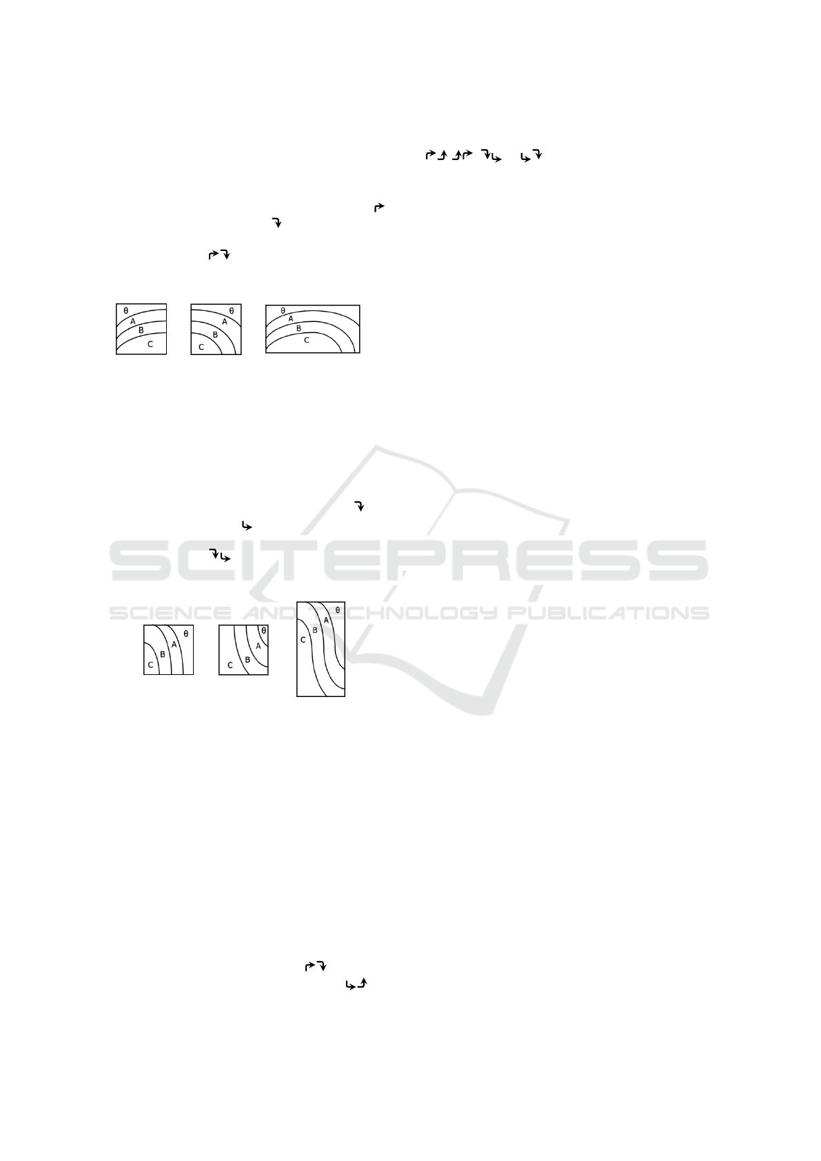
(a) original data (b) π/2 rotation
( (Aθ)()(ABC)(B), ) ( (B)(Aθ)()(ABC), )
(c) flip horizontal (d) flip vertical
( (AB)(C)(BAθ)(), ) ( (BAθ)()(AB)(C), )
Figure 4: Operations on S
0
.
2. For each D in S
0
, f (D) is valid.
3. f ( f ( f ( f (D)))) = D.
Proof. This can easily be proved, since the operation
is only swapping segments.
Example 4. The representation for Figure 4(a) is
D = ((Aθ)()(ABC)(B), ). If we draw f (D) =
( (B)(Aθ)()(ABC), ), then we can obtain the model
shown in Figure 4(b), which corresponds to π/2
clockwisely rotated with respect to the original model
shown in Figure 4(a).
5.2 Horizontal Flip
Let g be the operation that flips the model horizon-
tally.
First, we detect the layer that is encountered last
on tracing the borderline of the model before apply-
ing the operation, that is, the layer which will occupy
the top-left corner of the model after applying the op-
eration. This is said to be a delimiter and is defined as
follows.
For L = (σ
t
)(σ
r
)(σ
b
)(σ
l
),
delimiter =



last(σ
t
) (if σ
t
6= ε)
last(σ
l
) (if σ
t
= ε, σ
l
6= ε)
last(σ
b
) (if σ
t
= σ
l
= ε).
Let I = e
1
...e
k
be the layer-sequence of L
and e
z
be the delimiter (1 ≤ z ≤ k). Let I
0
=
e
z−1
e
z−2
...e
1
e
k
e
k−1
...e
z
.
Then we set g(L) = (σ
0
t
)(σ
0
r
)(σ
0
b
)(σ
0
l
), by divid-
ing I
0
into four segments by inserting the symbols ’(’
and ’)’ so that |σ
0
t
| = |σ
t
|, |σ
0
r
| = |σ
l
|, |σ
0
b
| = |σ
b
| and
|σ
0
l
| = |σ
r
|.
For C, g( ) = ,g( ) = ,g( ) = ,g( ) = .
Proposition 3. 1. The model corresponding to g(D)
is a figure that is horizontally flipped relative to
that corresponding to D.
2. For each D in S
0
, g(D) is valid.
3. g(g(D)) = D.
Proof. 1. Considering cyclicity, I
0
= I
−1
. The en-
countered order of layers on tracing the borderline
of the model for g(L) is the inverse of that in the
original model. Moreover, the numbers of end-
points on each side of the original model are the
same as on the corresponding sides of the model
for g(L), since |σ| indicates the number of end-
points on the side σ.
2. Assume that L is valid.
I
0
= I
−1
. In addition, for any pair X and Y of
layer-symbols chgpt(X/Y,σ) and chgpt(Y /X, σ
0
)
are mapped to chgpt(Y /X, τ) and chgpt(X/Y,τ
0
),
respectively, by g. Then τ 6= τ
0
holds since σ 6= σ
0
holds, from the definition of g. Therefore, validity
[v1] holds.
Validity [v2] holds, since I
0
= I
−1
.
Validity [v3] trivially holds.
We show that validity [v4] holds as follows. We
show the case of C ∈ Dn. Since the inclinations
of all the layer-borderlines are either dn or any,
we consider a case in which chgpt(X /Y, σ
b
)
and chgpt(Y /X, σ
l
) hold where the inclination
is C
XY
= dn. In this case, the pair of these
end-points is mapped to the pair chgpt(Y /X, σ
0
b
)
and chgpt(X/Y, σ
0
r
), respectively, by g. Their
inclination is up. Similarly, for the other layer-
borderlines, the inclination of dn is mapped to
up, and any to any. Therefore, g(C) ∈ U p holds.
It follows that validity [v4] holds in this case. We
can prove the other cases similarly.
3. g(g(D)) = D holds trivially.
Example 5. The representation for the model in Fig-
ure 4(a) is D = ((Aθ)()(ABC)(B), ). If we draw
g(D) = ((AB)(C)(BAθ)(), ), then we can obtain the
model shown in Figure 4(c), which corresponds to
the horizontally flipped original model shown in Fig-
ure 4(a).
5.3 Vertical Flip
Let h be the operation that flips the model vertically.
In this case, the delimiter is defined as follows.
For L = (σ
t
)(σ
r
)(σ
b
)(σ
l
),
delimiter =



last(σ
b
) (if σ
b
6= ε)
last(σ
r
) (if σ
b
= ε, σ
r
6= ε)
last(σ
t
) (if σ
b
= σ
r
= ε).
Let I = e
1
...e
k
be the layer-sequence of L
and e
z
be the delimiter (1 ≤ z ≤ k). Let I
0
=
e
z−1
e
z−2
...e
1
e
k
e
k−1
...e
z
.
Qualitative Spatial Representation and Reasoning About Fold Strata
215

Then we set h(L) = (σ
0
t
)(σ
0
r
)(σ
0
b
)(σ
0
l
), by divid-
ing I
0
into four segments by inserting the symbols ’(’
and ’)’ so that |σ
0
t
| = |σ
b
|, |σ
0
r
| = |σ
r
|, |σ
0
b
| = |σ
t
| and
|σ
0
l
| = |σ
l
|.
For C, h( ) = , h( ) = ,h( ) = ,h( ) = .
Proposition 4. 1. The model corresponding to h(D)
is a figure that is vertically flipped relative to that
corresponding to D.
2. For each D in S
0
, h(D) is valid.
3. h(h(D)) = D.
Proof. Similar to the proof of g.
Example 6. The representation for Figure 4(a) is
D = ((Aθ)()(ABC)(B), ). If we draw h(D) =
( (BAθ)()(AB)(C), ), then we can obtain the model
shown in Figure 4(d) that corresponds to the verti-
cally flipped original model shown in Figure 4(a).
5.4 Combination of Operations
Proposition 5. For D
1
,D
2
∈ S
0
where D
1
= (L
1
,C
2
)
and D
2
= (L
2
,C
2
), if D
2
can be obtained from D
1
by
applying the operations f ,g and h finite times, then
the layer-sequences of L
1
and L
2
are equivalent.
Proof. Let L
1
= (σ
t
)(σ
r
)(σ
b
)(σ
l
). Then layer-
sequence of L
1
is I = σ
t
σ
r
σ
b
σ
l
.
The layer-sequence of f (L
1
) = (σ
l
)(σ
t
)(σ
r
)(σ
b
) is
σ
l
σ
t
σ
r
σ
b
, which is equivalent to I because of its
cyclicity.
The layer-sequences of g(L
1
) and h(L
1
) are equiv-
alent to I
0
= e
z−1
e
z−2
...e
1
e
k
e
k−1
...e
z
, where e
z
is
the delimiter of L
1
. Therefore, they are equivalent to
I.
The following property holds with respect to the
combination of the operations, which can be easily
proved.
Proposition 6. f ( f (D)) = g(h(D)) = h(g(D)).
6 REASONING
6.1 Interconnection of Models
For a pair of representations for models, if the ad-
jacency between the layers appearing in them is the
same, then their configuration is the same.
Definition 5 (same configuration). For a pair of
representations for models D
1
= (L
1
,C
1
) and D
2
=
(L
2
,C
2
), let I
1
and I
2
be layer-sequences of L
1
and
L
2
, respectively. If I
1
= I
2
, then it is said that D
1
and
D
2
have the same configuration.
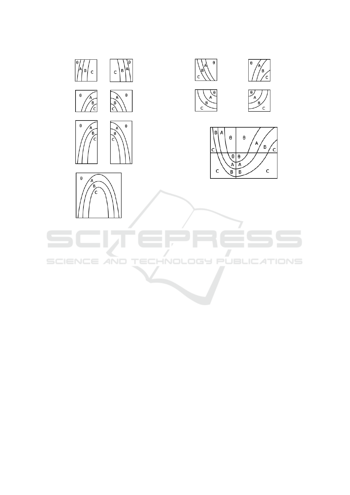
Example 7. In Figure 5, (a), (b) and (c) have the
same configuration, whereas (d) does not.
(a) (Aθ)()(ABC)(B) (b) ()(ABC)()(BAθ)
(c) ()(ABC)(BAθ)() (d) (Bθ)(B)(CA)(C)
Figure 5: Same/different configuration.
Let S
0
be a set of representations for models of
local data. When D
1
,D
2
∈ S
0
have the same configu-
ration, we make a new model D by connecting them
horizontally or vertically.
First, we discuss horizontal connection.
For a pair of D
1
= (L
1
,C
1
) and D
2
= (L
2
,C
2
) in S
0
that have the same configuration, we can connect the
right side of D
1
to the left side of D
2
if the following
two conditions are satisfied.
[Conditions for horizontal connection]
1. Let L
1
= (σ
t
)(σ
r
)(σ
b
)(σ
l
) and L
2
=
(τ
t
)(τ
r
)(τ
b
)(τ
l
). Take elements c
i
of the
sequence-of-transitions of L
1
that satisfy
chgpt(c
i
,σ
r
), and put them in the order of
their appearance to make the sequence c
1
...c
k
.
Similarly, take elements c
0
j
of the sequence-of-
transitions of L
2
that satisfy chgpt(c
0
j
,τ
l
), and put
them in their order of appearance to make the
sequence c
0
1
...c
0
k
0
. Then k = k
0
= |L
1
|/2 = |L
2
|/2,
and if c
i
= e
i−1
/e
i
then c
0
i
= e
k+1−i
/e
k−i
for each
i (1 ≤ i ≤ k).
2. Either of the following holds.
(a) last(C
1
), f irst(C
2
) ∈ U p
(b) last(C
1
), f irst(C
2
) ∈ Dn
(c) last(C
1
) =
and f irst(C
2
) =
(d) last(C
1
) = and f irst(C
2
) =
The first condition means that all the end-points
occurring on two connecting sides coincide, and that
all the layer-symbols appear on both connecting sides.
This avoids the case in which the figure correspond-
ing to the resulting representation could contain a dis-
connected region. We explain this later. The second
condition means that the shapes of all the connected
layer-borderlines are smooth.
If both conditions are satisfied, then we can con-
nect D
1
and D
2
to generate the representation D =
ICAART 2023 - 15th International Conference on Agents and Artificial Intelligence
216

(L,C). L = (σ
t
τ
t
)(τ
r
)(τ
b
σ
b
)(σ
l
). C is the sequence of
shape-symbols obtained by replacing qq, a repetition
of shape-symbols, in C
1
C
2
by q for each q ∈ Lang2.
Example 8. The representations for the models in
Figure 6(a) and (b) are D
1
= ( ()(ABC)()(BAθ), )
and D
2
= ( ()(A)(BC)(BAθ), ), respectively, and
their horizontal connection is computed as D
1
||D
2
=
( ()(A)(BC)(BAθ), ) which is the representation
for the model in Figure 6(c).
(a) D
1
(b) D
2
(c) D
1
||D
2
Figure 6: Horizontal connection.
Vertical connection can be defined similarly; con-
necting the lower side of D
1
and the upper side of D
2
,
which is denoted by D
1
+D
2
, when D
1
and D
2
satisfy
the conditions on vertical connection.
Example 9. The expressions for the models in Fig-
ure 7(a) and (b) are D
1
= ( (Aθ)()(ABC)(B), ) and
D
2
= ( (BAθ)(AB)(C)(), ), respectively, and their
vertical connection can be computed as D
1
+ D
2
=
( (Aθ)(AB)(C)(B), ) which is the expression for
the model of Figure 7(c).
(a) D
1
(b) D
2
(c) D
1
+ D
2
Figure 7: Vertical connection.
We define S
1
as a union of the set of representa-
tions for the horizontally/vertically connected models
and S
0
.
S
1
= { D | D = D
1
||D
2
,D
1
,D
2
∈ S
0
}
∪ { D | D = D
1
+ D
2
,D
1
,D
2
∈ S
0
}
∪ S
0
.
We repeat this process by generating S
n
from S
n−1
for n > 1.
S
n
= { D | D = D
1
||D
2
,D
1
,D
2
∈ S
n−1
}
∪ { D | D = D
1
+ D
2
,D
1
,D
2
∈ S
n−1
}
∪ S
n−1
.
For the representation (L,C) ∈ S
n
, we can extract
the characteristics of the shape of layer-borderlines
from C: if C includes a sub-sequence , then it has a
maximal point; if C includes a sub-sequence , then
it has a minimal point; if C includes a sub-sequence
, , or , then it has an inflection point.
In general, D ∈ S
n
is not always a valid represen-
tation, since a layer-borderline of D may include an
extremum or inflection. Instead, the following prop-
erties hold.
Theorem 3 (property of extended representation).
D = (L,C) ∈ S
n
satisfies the following properties.
Let L = (σ
t
)(σ
r
)(σ
b
)(σ
l
), the layer-sequence of
L, I = e
1
...e
k
and C = q
1
,...,q
t
.
p1: For any pair X and Y of layer-symbols, if L in-
cludes chgpt(X/Y, σ), then it includes exactly one
chgpt(Y /X,σ
0
), where σ, σ
0
∈ {σ
t
,σ
r
,σ
b
,σ
l
}.
p2: I is X
n
θ or in the form X
1
...X
n−1
X
n
X
n−1
...X
1
θ,
where X
i
6= X
j
(1 ≤ i < j ≤ n).
p3: For any i (1 ≤ i ≤ t − 1), q
i
6= q
i+1
holds.
We can apply a combination of horizontal/vertical
connection to obtain the sequence S
0
,S
1
,...,S
n
.
However, we have to choose the order of application
because of the conditions of the connection.
Example 10. In Figure 8, D
1
and D
2
cannot be
horizontally connected, since they do not satisfy the
first condition of horizontal connection. On the other
hand, D
3
+ D
1
and D
4
+ D
2
can be generated since
the pair D
3
and D
1
, and the pair D
4
and D
2
satisfy the
conditions of vertical connection, respectively. In ad-
dition, (D
3
+ D
1
)||(D
4
+ D
2
) can be generated since
D
3
+ D
1
and D
4
+ D
2
satisfy the conditions of hori-
zontal connection.
As a result, a representation for the global data
that may contain a maximal point is obtained.
This example means that the properties stated in
Theorem 3 are preserved on applying the connections
in an appropriate order.
6.2 Prediction of Global Data
When multiple data are collected at distant locations,
if they have the same configuration, then we can
find several possible ways to connect them, using the
above reasoning.
Example 11. Assume that D
1
and D
2
are given, and
were collected at distant locations (Figure 9(a)), does
a global stratum exist that contains both of them? One
is shown in Figure 9(b), which shows that there exist
D
3
and D
4
to connect D
1
and D
2
. Such intermediate
data are often missing, and we infer the possibility
that the global stratum in Figure 9(b) exists, which
changes in the long term as a result of crustal move-
ments.
Qualitative Spatial Representation and Reasoning About Fold Strata
217

D
1
D
2
D
3
D
4
D
3
+ D
1
D
4
+ D
2
(D
3
+ D
1
)||(D
4
+ D
2
)
Figure 8: Operation process.
In this example, the right two rectangles are wider
than the left ones in Figure 9(b). Actually, the sizes of
collected local data are not always same or distances
between their locations are different. Here, we fo-
cus on the end-points of layer-borderlines and their
shapes both of which are treated qualitatively. There-
fore, we can make a model for a global data by chang-
ing the size or ratio of sides of rectangles of the mod-
els for local data.
Simple fold forms can be generated by connect-
ing multiple local data. This means that we can infer
the shape and structure of global data from a set of lo-
cal data collected in different locations. Currently, the
connection conditions are too strict to generate com-
plex fold forms. We will revise the conditions in fu-
ture studies.
7 RELATED WORKS
To the best of the authors’ knowledge, there has been
almost no research on strata that uses symbolic repre-
sentation and logical reasoning.
To combine AI techniques and structural geology,
application of machine learning using big data is one
possibility. However, the currently available strata-
data archives are quite small and the stored data are
D
1
D
2
D
3
D
4
(a) local data
(b) global data
Figure 9: Prediction of globald data.
not sufficiently categorized. Moreover, in most data
archives, figures and landscapes are stored using nu-
merical data.
On the other hand, in the QSR research field, sev-
eral methods for symbolic treatment of shapes have
been proposed. Almost all of them treat spatial data
on a two-dimensional plane.
Leyton proposed a grammar that represents
changes in the shape of a closed curve, starting from a
simple smooth curve. He explained changes in shape
based on a force acting from inside or outside the
curve (Leyton, 1988). He showed that any shape of
a smooth closed curve can be represented using lan-
guage based on the proposed grammar. Tosue et al.
extended the grammar so that it can represent phe-
nomena such as the creation of a tangent point and
division of the curve (Tosue and Takahashi, 2019).
They applied the method to a process of organogene-
sis. Galton et al. proposed another grammar that can
apply to not only a smooth curve but also to a straight
line or a curve with cusps (Galton and Meathrel,
1999). They showed that objects of various shapes
can be symbolically represented by connecting a fi-
nite number of primitive segments. They also re-
ferred to transformation between representations dif-
fering in granularity. Cabedo et al. proposed a rep-
resentation for the borderline of an object with fur-
ther information such as relative lengths and relative
angles, and also showed the juxtaposition of objects
(Cabedo and Escrig, 2004; Cabedo et al., 2010; Pich
and Falomir, 2018), and Falomir et al. defined sim-
ilarity between qualitative shapes described in their
extended model (Falomir et al., 2013).
ICAART 2023 - 15th International Conference on Agents and Artificial Intelligence
218

All of these expressions adopted methods that rep-
resent the shape of an object by connecting primitive
segments when tracing its borderline. On the other
hand, Cohn took a different, approach to represent
a concave object (Cohn, 1995). He regarded differ-
ences in the closure and the object itself as regions
and represented the spatial relations of these regions.
Kumokawa et al. also proposed a different represen-
tation for a concave shape using closure (Kumokawa
and Takahashi, 2008).
A study by Kulik et al. applied QSR to landscape
silhouettes (Kulik and Egenhofer, 2003). They pro-
posed a description language for the shape of an open
line. They defined several primitives comprising two
consecutive vectors depending on relative lengths and
angles; regarded the borderline of a silhouette of a
landscape as a pattern of connections between these
primitives; and deduced landscape features, including
mountain, valley, and plateau. They also proposed a
transformation from the refined level to the abstract
level. The differences between Kulik’s method and
ours are: first, he used straight lines as primitives,
whereas we use curves; second, his target silhou-
ette was always in the vertical direction, whereas our
method can be applied to rotated forms; third, he nei-
ther formalized the method nor discussed the validity
of the representation, whereas we both define the va-
lidity of the representation and prove one-to-one rela-
tion with the model.
In addition, whereas all extant studies treated the
essentially one-dimensional data of a borderline, we
treated the two-dimensional data of a stratum consist-
ing of multiple regions.
8 CONCLUSIONS
We have discussed qualitative representation and rea-
soning for strata.
We developed a model for local data from a typ-
ical fold, and proposed its representation in the form
of a pair of sequences of symbols that stand for the
configuration of a layer and the shapes of the border-
lines between layers. This representation is suitable
to show the main features of strata: one layer extends
in one direction if there is no fault, and the relations of
interconnections between layers are unchanged even
if the width of a layer, shape, or axis of a fold changes.
We defined the required validity of the representa-
tion, and then showed that the valid representation and
that of the model have a one-to-one relation. More-
over, we defined several operations on the represen-
tation, and showed that they preserve its validity. We
also showed that global data can be generated by con-
necting local data with the same configuration. This
enables derivation of relations among multiple local
data collected in different locations or at different
times. Our main contribution is to show symbolic
treatment of strata and provide a basis for logically
explaining the process of landscape generation.
In future studies, we intend to identify sets of rep-
resentations obtained from repetitive application of
connections of local data. We are also considering the
formalization needed to explain the strata-generation
process, as well as a qualitative simulation for possi-
ble future morphological changes.
ACKNOWLEDGEMENTS
This research is supported by JSPS Kakenhi
JP21K12020. The authors would like to thank Mo-
tohiro Tsuboi for giving useful advice from the field
of geology.
REFERENCES
Cabedo, L. M., Abril, L. G., Morente, F. V., and
Falomir, Z. (2010). A pragmatic qualitative ap-
proach for juxtaposing shapes. Journal of Uni-
versal Computer Science, 16(11):1410–1424.
Cabedo, L. M. and Escrig, M. T. (2004). A qualita-
tive theory for shape representation and match-
ing for design. Proceedings of the Sixteenth
Eureopean Conference on Artificial Intelligence,
ECAI’2004, pages 858–862.
Chen, J., Cohn, A. G., Liu, D., Wang, S., Ouyang, J.,
and Yu, Q. (2013). A survey of qualitative spa-
tial representations. The Knowledge Engineering
Review, 30:106–136.
Cohn, A. and Renz, J. (2008). Qualitative spatial
representation and reasoning. In Handbook of
Knowledge Representation, chapter 13. Elsevier.
Cohn, A. G. (1995). Hierarchical representation of
qualitative shape based on connection and con-
vexity. Spatial Information Theory: Cognitive
and Computational Foundations of Geographic
Information Science (COSIT95), pages 311–326.
Falomir, Z., Abril, L. G., Cabedo, L. M., and Ortega,
J. A. (2013). Measures of similarity between
objects based on qualitative shape descriptions.
Spatial Cognition & Computation, 13(3):181–
218.
Galton, A. and Meathrel, R. (1999). Qualitative out-
line theory. Proceedings of the Sixteenth Inter-
Qualitative Spatial Representation and Reasoning About Fold Strata
219

national Joint Conference on Artificial Intelli-
gence, pages 1061–1066.
Kano, K. and Murata, A. (1998). Structural Geology.
Asakura Publishing Co., Ltd. (in Japanese).
Kulik, L. and Egenhofer, M. J. (2003). Linearized
terrain: languages for silhouette representations.
Spatial Information Theory. Foundations of Geo-
graphic Information Science, International Con-
ference, COSIT 2003, pages 118–135.
Kumokawa, S. and Takahashi, K. (2008). Qualitative
spatial representation based on connection pat-
terns and convexity. AAAI08 Workshop on Spa-
tial and Temporal Reasoning, pages 40–47.
Leyton, M. (1988). A process-grammar for shape.
Artificial Intelligence, 34:213–247.
Ligozat, G. (2011). Qualitative Spatial and Temporal
Reasoning. Wiley.
Pich, A. and Falomir, Z. (2018). Logical composi-
tion of qualitative shapes applied to solve spa-
tial reasoning tests. Cognitive Systems Research,
52:82–102.
Sioutis, M. and Wolter, D. (2021). Qualitative spatial
and temporal reasoning: current status and future
challenges. Proceedings of 30th International
Joint Conference on Artificial Intelligence, pages
4594–4601.
Tosue, M. and Takahashi, K. (2019). Towards a qual-
itative reasoning on shape change and object di-
vision. In Spatial Information Theory. 11th In-
ternational Conference, COSIT 2019, pages 7:1–
7:15.
ICAART 2023 - 15th International Conference on Agents and Artificial Intelligence
220