YOLO: You Only Look 10647 Times

Christian Limberg

1 a

, Andrew Melnik

, Helge Ritter

and Helmut Prendinger

National Institute of Informatics (NII), Tokyo, Japan

Bielefeld University, Bielefeld, Germany

Keywords:

Object Detection, Explainable AI/ML, YOLO, You Only Look Once.

Abstract:

In this work, we explore the You Only Look Once (YOLO) single-stage object detection architecture and com-

pare it to the simultaneous classiﬁcation of 10647 ﬁxed region proposals. We use two different approaches

to demonstrate that each of YOLO’s grid cells is attentive to a speciﬁc sub-region of previous layers. This

ﬁnding makes YOLO’s method comparable to local region proposals. Such insight reduces the conceptual gap

between YOLO-like single-stage object detection models, R-CNN-like two-stage region proposal based mod-

els, and ResNet-like image classiﬁcation models. For this work, we created interactive exploration tools for a

better visual understanding of the YOLO information processing streams: https://limchr.github.io/yolo_visu

1 INTRODUCTION

Much progress in detecting multiple objects in an im-

age using deep neural networks can be attributed to

the introduction of R-CNN (Girshick et al., 2014),

SSD (Liu et al., 2016), and YOLO (Redmon et al.,

2016) architectures. R-CNN and its improved ver-

sions like FasterRCNN (Ren et al., 2016) detect ob-

jects by ﬁrst producing proposals for regions contain-

ing an object (Melnik et al., 2021), and then in a sec-

ond stage these proposals get passed through a classi-

ﬁer network. YOLO and SSD work without a sep-

arate proposal stage by combining object detection

and classiﬁcation into one stage. Four YOLO archi-

tecture successors along with other one-stage models

were proposed. They introduce improvements such

as the usage of anchor boxes, separate pathways for

different object sizes, deeper architectures, different

activation functions and a variety of other tricks and

tweaks (Redmon and Farhadi, 2016), (Redmon and

Farhadi, 2018), (Bochkovskiy et al., 2020).

We argue that the performance of these systems

can be understood as performing classiﬁcation and

regression tasks for a high number of ﬁxed region

proposals with their positions relating to the convolu-

tional grid. To this end, we implement several interac-

tive visualizations, that (i) show the inner processing

of the network and (ii) provide detailed insights how

YOLO achieves both high speed and high accuracy.

In this paper we obtain insights of the inner me-

chanics of YOLO by modifying two distinct visual-

https://orcid.org/0000-0002-4903-3933

ization approaches that were originally developed for

examining classiﬁcation CNNs, and are here adapted

and applied for the YOLO object detection model.

The ﬁrst approach produces a saliency measure mo-

tivated by GradCam (Selvaraju et al., 2017). The sec-

ond approach is motivated by Inceptionism and Deep-

Dream (Mordvintsev et al., 2015) and optimizes the

input pattern that is fed into YOLO for matching a

speciﬁc target output response.

Both approaches use gradients for visualizing

characteristics of the network. In GradCam, we feed

an image with a target object into the network and

multiply activation and gradient in a particular inter-

mediate layer. On the other hand, in DeepDream we

are searching for optimal input patterns for minimiz-

ing a certain cost function on the prediction. In other

words, the input image itself is optimized in such a

way that the related output neuron response will get

closer to a desired target value.

The core ﬁndings of examining the modiﬁed ver-

sions of GradCam and DeepDream are:

• YOLO’s high-conﬁdence grid cells are sparse;

• each of YOLO’s grid cells is attentive to a variable

and localized sub-region of the input image;

• YOLO’s attention is variable and directly related

to the output neuron of interest;

• optimal input samples can be generated that opti-

mize speciﬁc target outputs. This can be used for

explaining the trained features responsible for de-

tecting objects of e.g. a speciﬁc class, position or

shape;

Limberg, C., Melnik, A., Ritter, H. and Prendinger, H.

YOLO: You Only Look 10647 Times.

DOI: 10.5220/0011677300003417

In Proceedings of the 18th International Joint Conference on Computer Vision, Imaging and Computer Graphics Theory and Applications (VISIGRAPP 2023) - Volume 5: VISAPP, pages

153-160

ISBN: 978-989-758-634-7; ISSN: 2184-4321

 2023 by SCITEPRESS – Science and Technology Publications, Lda. Under CC license (CC BY-NC-ND 4.0)

153

• we can understand YOLO as performing paral-

lelized classiﬁcation and regression tasks of many

image sub-regions. These regions efﬁciently

share most of their computation, resulting from a

high amount of overlap in CNNs.

By a simple post-processing step, only a very

sparse selection of YOLO’s output neurons are con-

sidered for the actual prediction, and the result

of most output neurons is simply ignored. For

YOLO.v4, the detection of a picture leads to a total

number of 10647 classiﬁcation/regression pairs, ob-

tained by summing up the squared grid shapes times

the number of anchor boxes ((13

+ 26

+ 52

) ∗ 3).

This number is dependent on the image dimensions

used for train YOLO.v4 which is 416x416 pixels. It

has to be adapted for other image dimensions, since

the dimensions of the grids would also change, if we

assume the same network architecture.

This article is organized as follows: In Section 2

we explain the YOLO.v4 architecture and discuss its

main principles. In Section 3 we introduce our ﬁrst

interactive visualizations of YOLO. Then we intro-

duce the adapted GradCam in Section 3.1 and Deep-

Dream approach in Section 3.2. Finally, in Section 4,

we draw our conclusion and point out some analogies

of YOLO’s computational strategy to computational

structures found in biological vision, where a good

trade-off between speed and accuracy is tantamount

as well.

2 YOLO ARCHITECTURE

In our experiments, we used a TensorFlow imple-

mentation

of YOLO.v4 (Bochkovskiy et al., 2020)

that uses the original weights. Other YOLO imple-

mentations can be found here: YOLO.v1-v3

and

YOLO.v5

. While there are newer versions of YOLO

out, YOLO.v4 was an optimal choice based on per-

formance, architecture clarity and code-availability.

However, our experiments should be reproducible for

following YOLO versions.

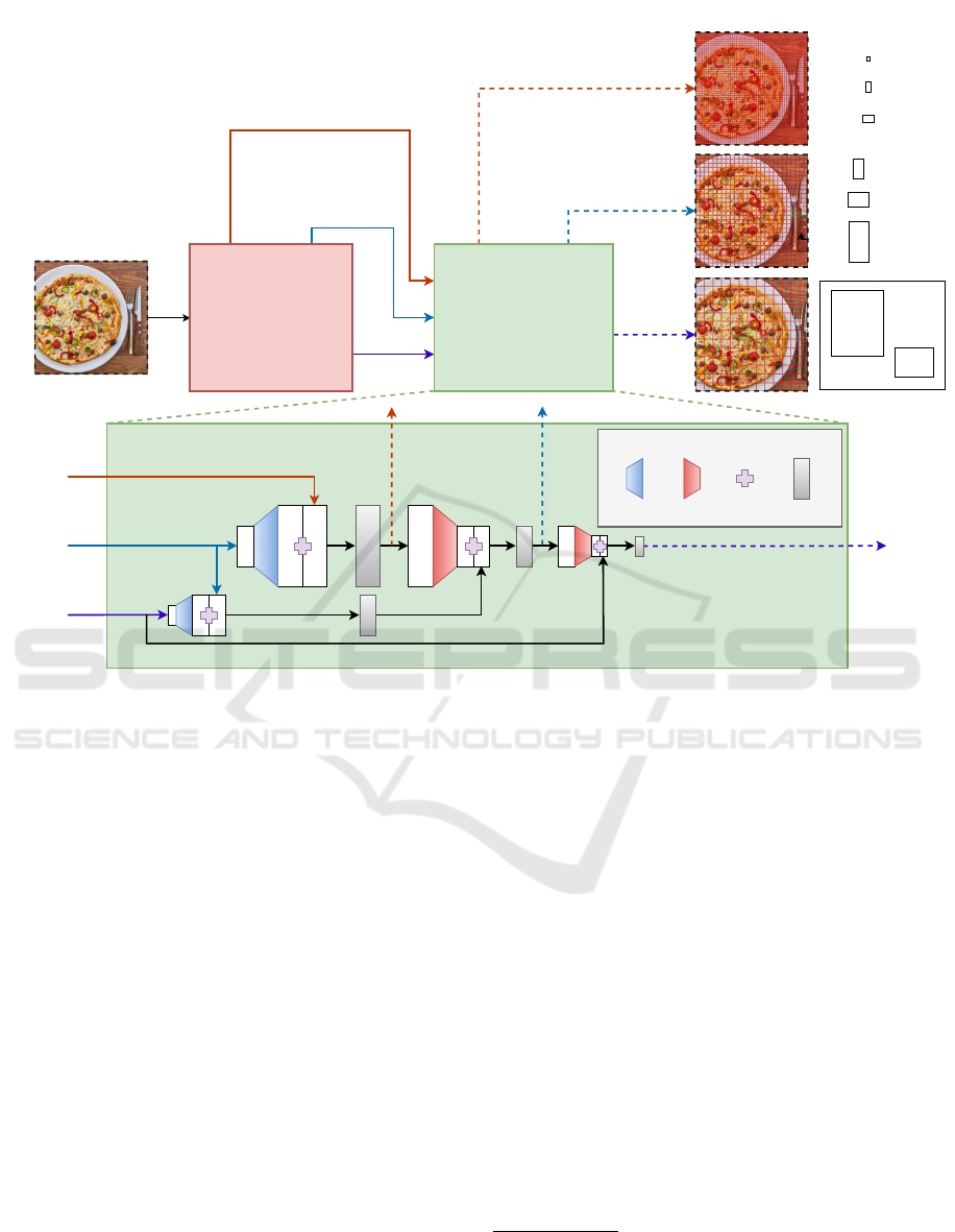
The network architecture is divided into two parts

(see Fig. 1): First, the image is processed by a back-

bone network for feature extraction and second, the

YOLO head is calculating object bounding boxes.

https://github.com/hunglc007/tensorflow-yolov4-tﬂite

https://pjreddie.com/darknet/yolo/

https://github.com/ultralytics/yolov5

2.1 Backbone Network

In YOLO.v4, darknet53 is used as a backbone for

feature extraction. The network assumes input rgb-

images of size (416 : 416). It consists of 23 residual

blocks and 77 convolutional layers. Five of the con-

volutional layers downsample the input by applying

strides of 2. The backbone’s output feature map and 2

intermediate outputs (after the fourth and ﬁfth down-

sampling steps) are then passed into the YOLO.v4

head.

2.2 YOLO Head

The YOLO head consists of 31 convolutions with a

stride of 1 and padding for ensuring the same output

size. Also, the three different paths from the backbone

are concatenated in the YOLO head at different points

with upsampling and downsampling operations (see

Fig. 1).

The YOLO.v4 head has 3 different output path-

ways supporting the detection of smaller, medium and

larger sized objects.

The ﬁrst output from the YOLO head is the small

objects pathway after 2 upsampling operations and

2 concatenations with all paths of the backbone net-

work. After another downsampling and concatena-

tion with skip-connection, the medium objects path-

way is deﬁned and after a last downsampling paired

with a concatenation, the ﬁnal output of the large ob-

jects pathway is deﬁned.

2.3 Anchor Boxes

Anchor boxes are predeﬁned bounding box patterns

used by YOLO to delineate regions for object candi-

dates. Each of YOLO’s three pathways uses 3 dif-

ferent anchor box patterns (9 in total, see Fig. 1 right

column). Each pathway further provides a grid of dif-

ferent resolutions (52x52x255 for small, 26x26x255

for medium, and 13x13x255 for large sized objects).

Each grid cell is estimating the 3 respective anchor

boxes. Each anchor box has 85 channels (summing

up to 255 channels per grid cell). Five of the 85 chan-

nels (x,y,w,h,c) represent the x- and y-displacement of

the center of the object’s bounding box, the width and

height of the bounding box and a conﬁdence value de-

noting that the speciﬁc anchor box is detecting an ob-

ject. p denotes the remaining 80 channels that are rep-

resenting a probability value for each of the 80 classes

for the COCO dataset.

The YOLO architecture can also be trained on a

dataset with an arbitrary number of classes. Then p

will denote the number of classes in the dataset. For

VISAPP 2023 - 18th International Conference on Computer Vision Theory and Applications

154

large pathway

13x13x255

Output Heads Anchor Boxes

Backbone Network

conv layers 0-77

downsampling with strides

YOLO Head

conv layers 78-109

(depicted below)

YOLO Head

416x416x3

52x52x256

26x26x512

13x13x512

small pathway

52x52x255

255 channels = 85 * 3 anchors

85 = 5 XYWHC neurons + 80 class

probabilities

(the same for medium and large pathways)

medium pathway

26x26x255

5 5

small pathway

52x52x255

medium pathway

26x26x255

52x52x256

26x26x512

13x13x512

large pathway

13x13x255

upsampling

downsampling

channel-wise

concatenation

block of

5 conv layers

12x16

19x36

40x28

36x75

76x55

72x146

142x110

192x243

459x401

Figure 1: A simpliﬁed schematic of the YOLO.v4 network architecture.

example (Melnik et al., 2022) trained the YOLO ar-

chitecture to detect faces and classify each detected

face into 10 age classes (0-10 years old, 10-20, 20-30,

30-40, 40-50, 50-60, 60-70, 70-80, 80-90, 90-100).

For training, all bounding boxes from the COCO

dataset were assigned to one (or several) of the YOLO

anchor boxes, based on their Intersection over Union

(IoU) value with the box patterns (see Section 2.4 for

more details). Thus, after training, each of these 9 an-

chor boxes is trained to predict its own type of bound-

ing box shape. Thus, the learnt anchor boxes work

like templates for detecting objects of different sizes

and shapes. There is e.g. an anchor box for detecting

rather big, vertical-shaped objects and there is an an-

chor box for detecting smaller horizontal objects, etc.

The YOLO architecture has 3 anchor boxes per grid

cell, where the resolution of the grid changes with the

3 pathways. A conﬁdence value near 0 indicates that

no object was found located spatially within the grid

cell. In Section 2.4 we further discuss how the train-

ing signal for the different anchor boxes, i.e. their rep-

resenting neurons, is calculated.

2.4 Training

As explained in the previous section, the YOLO

network is trained to map a 416x416x3 input ar-

ray into three head output pathways (grids of shape

52x52x255, 26x26x255, and 13x13x255) to repre-

sent the input at appropriate discretization outputs for

“small”, “medium” and “large” objects, with each

grid cell specifying three 85-dimensional channels for

encoding 3 object bounding boxes. A grid cell can

also opt not to represent its maximum of three boxes

each channel that represents a box indicates this by

setting its c-variable to 1, thereby assigning meaning

for the remaining 4+80 x,y,w,h and p neurons. Oth-

erwise, if c=0, these components are not to be inter-

preted as specifying anything.

With this representation convention, any dataset

with images of annotated axis-aligned bounding

boxes that represent the outline of objects can be

straightforwardly translated into target values for

Note that the maximum of three representable boxes per

channel is not in any deep way related to the number of

three pathways - it is perfectly thinkable to specify YOLO

architectures where these numbers are chosen to differ.

YOLO: You Only Look 10647 Times

155

channel components of the three output pathways.

For each image and each bounding box label, the 3

differently sized grid cells at the spatial center of the

object are identiﬁed. Each grid cell can be represented

by 3 different anchor boxes. For training the network,

the anchor boxes getting a positive training signal (de-

scribed below) have to be identiﬁed.

The anchor boxes that have an IoU greater than

0.3 compared to the annotated object bounding boxes

from the dataset are chosen to get a positive training

signal. If there is no anchor box fulﬁlling this crite-

ria, the anchor box with the largest IoU is selected to

get the positive training signal. All positive anchor

boxes are getting non-zero encoded values in the re-

spective positions of the target vector used for train-

ing. They are getting a conﬁdence value of 1, encoded

values for x,y,w,h of the respective object bounding

box, and a soft 1-hot-encoded vector representing the

object class as p. All other ﬁelds in the target vector

are set to 0’s for “no object present”.

With the so-deﬁned target values the architecture

can be straightforwardly trained to model the input-

output relationship in the training data. This architec-

ture can be compared to an ensemble of output paths,

where each path is trained to detect the most appro-

priate bounding boxes (Bach et al., 2020).

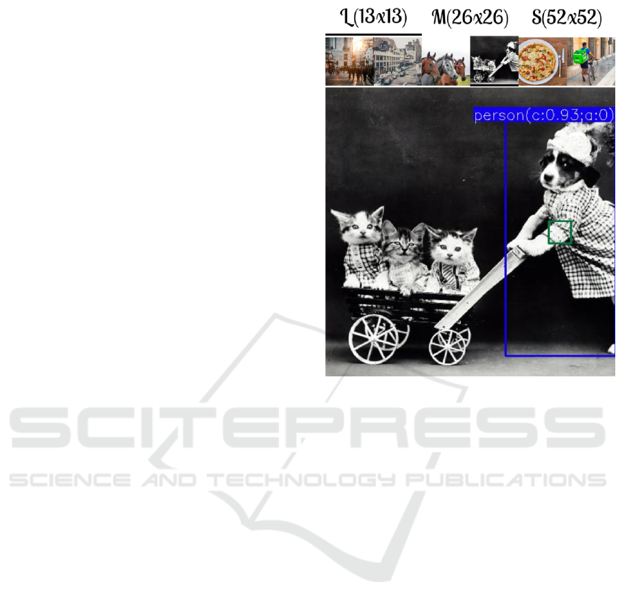
3 VISUALIZATION

For a deeper inquiry into the nature of the path-

way/grid cells representation that emerges under this

training in YOLO, we implemented an interactive vi-

sualization of all pathways/grid cells for several im-

ages (see Fig. 2).

The number of detectable objects is limited to

10647. However, also in a quite busy image with

many small objects covering the whole space (e.g.

Fig. 2 image 2), this number isn’t reached by far.

Since only a few anchor boxes get a non-zero training

signal, also the number of active (or high conﬁdent)

anchor boxes in a prediction step is rather sparse. In

fact, most of the anchor boxes are low-conﬁdence and

just “thrown away”. The few anchor boxes that have a

high conﬁdence are post processed and build the ﬁnal

detection result.

Fig. 3 depicts the conﬁdence mapping of a predic-

tion. By shifting the input image a few pixels, one

can see how the anchor boxes’ conﬁdences are also

shifting and an anchor box of a neighboring grid cell

“takes over”.

We ﬁnd that a maximum of 4 grid cells have a

high conﬁdence to detect a certain object, but most

of the time only 1 or 2 grid cells are active. Fig. 2

Figure 2: With our interactive visualization, the full grid

layers of the YOLO.v4 network can be depicted for several

images. The YOLO architecture has 3 different pathways

for recognizing objects of different sizes. The recognition

heads are located in 2d-grids of different resolutions. Each

grid element can detect underlying objects based of 3 pos-

sible anchor box shapes. Each anchor box reﬁnes estimates

of the x- and y-position, the width and the height, a conﬁ-

dence value and a probability vector of each class used for

training. The bounding boxes are labeled with the predicted

class, the certainty value and an index of the displayed an-

chor box (we depict only the most conﬁdent anchor box out

of the 3 possible). Object proposals with a high certainty

are colored blue. The interactive version of this plot can be

accessed via https://limchr.github.io/yolo_visu/index.html#

ﬁg2.

further shows that all of these active grid cells have

fairly similar bounding boxes, so as a post-processing

step an ordinary non-maximum suppression can be

applied, choosing the bounding box with the highest

conﬁdence.

3.1 Saliency-Based Analysis of YOLO

Layers

In this section we present an analysis of the re-

sponses of YOLO’s output pathways in terms of their

“saliency pattern” of an intermediate convolutional

layer. To compute a suitable saliency measure, we

build on the GradCam approach (Selvaraju et al.,

2017), which calculates gradients based on an out-

VISAPP 2023 - 18th International Conference on Computer Vision Theory and Applications

156

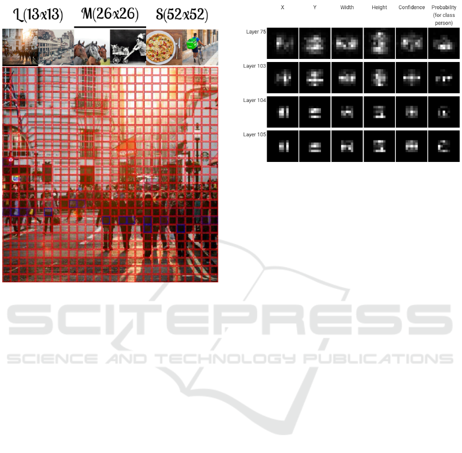
Figure 3: Shifting the actual input image below the grid

cells makes apparent how the conﬁdences of the anchor

boxes (blue means high conﬁdence) are shifted and neigh-

boring grid cells get activated. The interactive version of

this plot can be accessed via https://limchr.github.io/yolo_

visu/index.html#ﬁg3.

put neuron under consideration (e.g., typically a class-

neuron of the one-hot encoded output layer of a clas-

siﬁcation CNN).

To produce a scalar that indicates the importance

of a particular feature channel, the original algorithm

ﬁrst averages the gradients at the (usually last) con-

volutional layer over the spatial dimensions of the

layer’s channels. The scalar is then multiplied with

the actual activation values of neurons. The result

is an importance-weighted saliency map. The spatial

pattern of these values across the convolutional layer

and thus the corresponding input image shows which

input region is accountable for the response on the se-

lected output neuron.

For applying this technique to YOLO, we have to

make several changes. We can not use the very last

convolutional layer because of the different architec-

ture of the network (the last convolutional layers don’t

have that much saliency information because of the

grid outputs). Therefore, we use an intermediate layer

for computing saliency maps.

We found out that we can generate much more

descriptive saliency maps by multiplying the out-

put of the intermediate layer element-wise with the

Figure 4: Our adapted Detection GradCam visualizes the

saliency map of a single output neuron. The columns repre-

sent the saliency maps of the x-shift, y-shift, width, height,

conﬁdence and probability neuron of a selected grid cells of

the large pathway (13x13 grid). As rows, we depict saliency

maps for convolutional layers 75, 103, 104 and 105. Each

plot represents the saliency map averaged over 15 images

(15x13x13) having class “person” under the corresponding

grid cell’s position. The interactive version of this plot can

be accessed via https://limchr.github.io/yolo_visu/index.h

tml#ﬁg4.

plain gradients of this layer (e.g. calculated from

the w-neuron or the h-neuron of one speciﬁc grid

cell/anchor box) and average the output channels. But

still, the so-obtained result is pretty noisy. We did an-

other trick for getting a clearer pattern: We query sev-

eral images from the COCO dataset that have an in-

stance of a particular class (e.g. “person”) located at

a particular spatial image position, i.e. where the un-

derlying YOLO grid cell would get a positive train-

ing signal. We pass 15 of these images through our

adapted GradCam algorithm and average the result

images for getting a saliency map for this grid cell. By

repeating the process for all grid cells (omitting bor-

der grid cells since in the dataset are too few samples

having persons located in the border areas), we get a

clearer visualization and we can see how the saliency

of YOLO will shift as we hover over the image (see

Fig. 4).

The ﬁgure shows that the saliency is focused be-

low the corresponding grid cell’s position. Further,

it depicts that the saliency map of the w-neuron and

x-neuron has a rather wider activation, while the h-

neuron’s and y-neuron’s saliency map has a rather

vertical activation, i.e. the detection is more sensitive

to these areas. The activation of the p-neuron, which

is representing the class “human” in p) and especially

the c-neuron is more focused to the center.

YOLO: You Only Look 10647 Times

157

3.2 Optimization-Based Analysis of

YOLO Input Patterns

Back in 2014/2015, the Inceptionism and DeepDream

approaches (Mordvintsev et al., 2015) showed that

input images can be optimized for maximizing a

particular intermediate or output neuron of the net-

work. Those input images then show patterns that

the respective neurons are responsive to (Olah et al.,

2017). The optimization process is achieved by

forward-passing an image into the network and back-

propagating the gradients back into the input layer.

The input layer, or rather say, the subsequently chang-

ing input image, is then modiﬁed by adding the nor-

malized gradient multiplied by a optimization rate.

The weights of the neural network, however, are

frozen and do not change.

The main difference regarding detection models

is that we usually want to optimize for multiple out-

put neurons, since we can not only estimate the class

of the object but also its shape and position, which

relates to additional regression problems. In other

words, we not only want to maximize the stimulus of

a particular neuron of a one-hot encoded output layer

by gradient ascent, we are using a gradient descent ap-

proach for optimizing several of YOLO’s output neu-

rons to be a speciﬁc target value (e.g. the object’s

height should be 200 pixels). Doing this, we can re-

quire the target object to have a speciﬁc size and posi-

tion in the image simultaneously with optimizing for

speciﬁc features/classes.

In our experiments, we are starting the optimiza-

tion process with a grey image. The gradients are cal-

culated by considering all neurons of a speciﬁc grid

cell/anchor box to be a pre-deﬁned target value. We

set the conﬁdence neuron c and the target class’ p-

neuron of this anchor box to be optimized to be 1, all

other neurons in p are optimized to be 0. The x,y,w,h-

neurons can be set to be optimized to a speciﬁc target

value.

The target matrices have the shape of the 3 out-

put pathways and gradients are computed as the dif-

ference of target matrix and actual output values.

({13x13,26x26,52x52}x3x85). Other than directly

back-propagating these gradients through the net-

work, they are ﬁrst multiplied by a multiplier mask

that is weighting each output neuron. If we set the a

multiplier in that mask to a high value, the gradient of

the respective output neuron would be more inﬂuen-

tial to the optimization process. A value of 0 in the

multiplier mask would neglect the respective neuron.

We thereby give the c- and p-neuron of the positive

anchor box a weight of 10 each - making them more

inﬂuential regarding the update process. In our ex-

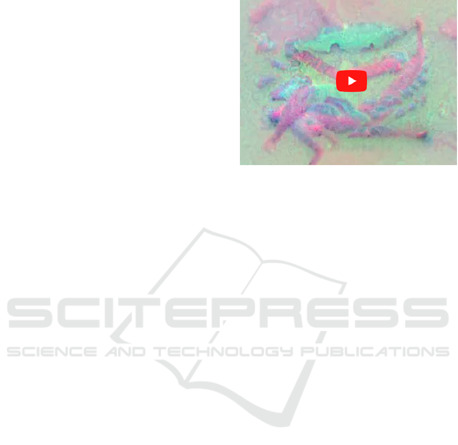
Figure 5: Video demonstrating the optimization process of

several classes of the COCO data set by our proposed “Deep

Detection Dream” approach. The video can be accessed via

https://limchr.github.io/yolo_visu/index.html#ﬁg5.

periments we set the target conﬁdences of all other

anchor boxes to 0 with a small multiplier. If we set

the multiplier of all other anchor boxes to 0, i.e. ig-

noring them for calculating the gradient, the process

would converge faster to the target class but may also

include other classes at random positions as well. As

loss function we use a weighted sum of the L

-loss

loss and the total variation score for reducing noise.

In classiﬁcation networks for reducing noise often

shift and/or rotation operations are applied to the in-

put image (Olah et al., 2017). However, we found out

that in detection networks this will affect the detec-

tion position so that the optimization process is not

converging well. Using the described method “Deep

Detection Dream” we created optimized input images

for several classes of the COCO data set used to train

YOLO. In Fig. 5 several of these optimization pro-

cesses are visualized for the center grid cell of the

large object pathway. The object’s target width and

height are 200 pixels each, this is 41% of the image

width/height.

Next, the capabilities to generate objects at a cer-

tain image position are illustrated. In Fig. 6 we are

optimizing an object for every grid cell. The result

is strongly resembling Fig. 4 and supports our claim

that each grid cell is attentive to its underlying image

area.

Not only the object class and position can be op-

timized towards a desired value but also the object’s

dimensions, i.e. its width and height. This can be ex-

plored by another interactive visualization in Fig. 7.

It can be seen that a non-matching conﬁguration

of output head and w,h target values is affecting the

result quality, i.e. generating small objects with the

large object head does not result in a well recogniz-

VISAPP 2023 - 18th International Conference on Computer Vision Theory and Applications

158

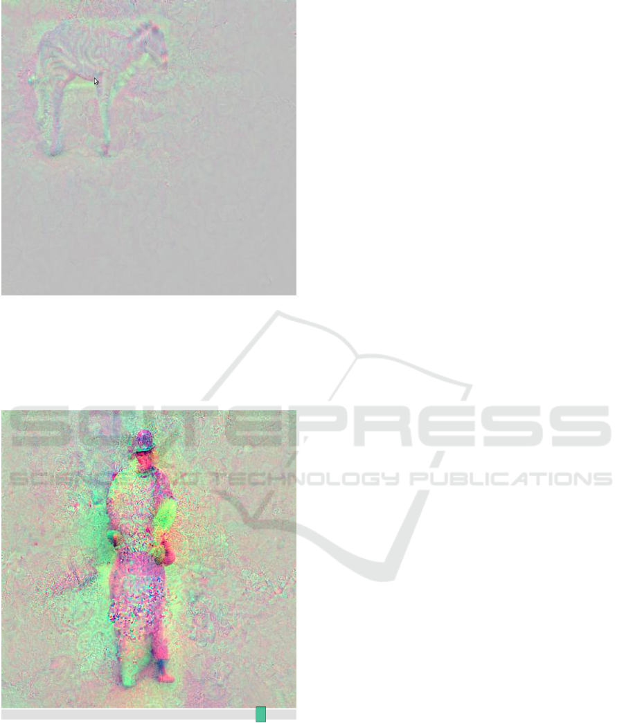
Figure 6: By our proposed “Deep Detection Dream” ap-

proach, we can generate objects in speciﬁc spatial image

regions. The static print ﬁgure can only show for a single

position speciﬁcation the associated sensitivity region. The

interactive version, accessible via https://limchr.github.io/y

olo_visu/index.html#ﬁg6, allows to explore the sensitivity

region as a function of an interactively chosen position.

Figure 7: By our proposed detection dream approach, we

can generate objects with speciﬁc attributes like in this case

an adjustable height. The interactive version of this plot can

be accessed via https://limchr.github.io/yolo_visu/index.h

tml#ﬁg7.

able images. Other experiments also showed, that if

the samples of a particular object class are usually

small in the images of the training data base, those

classes cannot reconstructed well with the big anchor

boxes neither.

However, Fig. 7 extends our statement to the effect

that the attentive image region is variable in size and

also shape.

4 CONCLUSION

The visualization of saliency patterns and optimized

input images of YOLO reveal that YOLO acts like

parallelized classiﬁcation CNNs: each anchor box’s

saliency is pointed to an underlying subarea of the

image and on this subarea classiﬁcation and regres-

sion tasks are focused. These tasks are locally inter-

dependent (the dimensions and location of a box are

determined by its contents and vice versa). However,

this tight spatial coupling focuses the propagation of

the gradients and their interactions, creating a strong

“spatial hierarchy”-bias that makes learning and sub-

sequent processing very efﬁcient.

This is not dissimilar to the information process-

ing in human visual cortex (Sheth and Young, 2016;

Melnik et al., 2018). In the primary visual cortex V1,

features are extracted and passed to secondary visual

cortex V2, where the information is split into a dorsal

and ventral stream for localizing (dorsal) and classi-

fying (ventral) objects. The dorsal stream is more ex-

plorative, showing a wider activation in the biological

saliency map for localizing objects and movements in

the scenery, where the ventral stream’s activation fo-

cuses more on the center of the object (see (Sheth and

Young, 2016) Fig. 2). We can see similar properties

also in Fig. 4, when comparing columns x,y,w,h with

c,p: x,y deﬁne the relative position of the detected

object and w,h represent the dimensions of the object.

I.e. the four neurons estimate where the object is,

while c and p determine if there is an object present,

and the object’s class (what is it?). The saliency map

activations of x,y,w,h is rather wide, focusing on the

object borders (x,w for horizontal and y,h for vertical

border areas) for determining where exactly it is, and

the activation of c,p is more narrow and focused to the

center, comparable to the dorsal and ventral stream of

the biological model.

The nature of an artiﬁcial neural network, and es-

pecially a CNN, is that it consists of many parallel

operations for one layer. This relates to a simple ma-

trix multiplication. GPUs are built for this purpose

and modern GPUs can do many matrix calculations

in a very short amount of time. So it seems natural to

exploit this feature and just “throw away the uninter-

esting results”, i.e. the low conﬁdence detections.

YOLO: You Only Look 10647 Times

159

Compared to early 2-stage detectors, which had

intermediate steps for selecting, e.g. region proposals

which were then fed into a second neural network,

the advantage is a massive speed increase (and only a

minor loss in accuracy) since this intermediate steps

take time since they are running on the CPU.

In this article, we demonstrated and visualized the

inner mechanics of the YOLO architecture. Our key

message is that YOLO is not really “looking once”,

but a lot more often. Because of a clever exploitation

of Artiﬁcial Neural Network structures, which make

it possible to share most of the computation between

regions and also allow to easily parallelize the compu-

tations on a GPU, this can be very fast and efﬁcient.

Our ﬁndings might be used for future develop-

ments in architecture design or for evaluating trained

models. Interesting future work include the improve-

ment of these visualization techniques. Also, the pro-

posed detection dream approach might be used to de-

termine how much information about a training image

is actually saved “within the weights of the network”

by setting the target output to the actual prediction

output of the model and optimize from a gray image.

Also, different other constraints can be added to the

optimization loss. By including the distance to a color

histogram into the loss function, the reconstructed im-

ages might can be improved to have a more realistic

color distribution.

ACKNOWLEDGEMENTS

This work was supported by a fellowship within the

IFI program of the German Academic Exchange Ser-

vice (DAAD).

REFERENCES

Bach, N., Melnik, A., Rosetto, F., and Ritter, H. (2020).

An error-based addressing architecture for dynamic

model learning. In International Conference on

Machine Learning, Optimization, and Data Science,

pages 617–630. Springer.

Bochkovskiy, A., Wang, C.-Y., and Liao, H.-Y. M. (2020).

Yolov4: Optimal speed and accuracy of object detec-

tion. arXiv preprint arXiv:2004.10934.

Girshick, R., Donahue, J., Darrell, T., and Malik, J. (2014).

Rich feature hierarchies for accurate object detec-

tion and semantic segmentation. In Proceedings of

the IEEE conference on computer vision and pattern

recognition, pages 580–587.

Liu, W., Anguelov, D., Erhan, D., Szegedy, C., Reed, S.,

Fu, C.-Y., and Berg, A. C. (2016). Ssd: Single shot

multibox detector. In European conference on com-

puter vision, pages 21–37. Springer.

Melnik, A., Akbulut, E., Sheikh, J., Loos, K., Buettner, M.,

and Lenze, T. (2022). Faces: Ai blitz xiii solutions.

arXiv preprint arXiv:2204.01081.

Melnik, A., Harter, A., Limberg, C., Rana, K., Sünderhauf,

N., and Ritter, H. (2021). Critic guided segmentation

of rewarding objects in ﬁrst-person views. In German

Conference on Artiﬁcial Intelligence (Künstliche In-

telligenz), pages 338–348. Springer.

Melnik, A., Schüler, F., Rothkopf, C. A., and König, P.

(2018). The world as an external memory: the price of

saccades in a sensorimotor task. Frontiers in behav-

ioral neuroscience, 12:253.

Mordvintsev, A., Olah, C., and Tyka, M. (2015). Inception-

ism: Going deeper into neural networks.

Olah, C., Mordvintsev, A., and Schubert, L. (2017). Feature

visualization. Distill. https://distill.pub/2017/feature-

visualization.

Redmon, J., Divvala, S., Girshick, R., and Farhadi, A.

(2016). You only look once: Uniﬁed, real-time object

detection. In Proceedings of the IEEE conference on

computer vision and pattern recognition, pages 779–

788.

Redmon, J. and Farhadi, A. (2016). Yolo9000: Better,

faster, stronger.

Redmon, J. and Farhadi, A. (2018). Yolov3: An incremental

improvement.

Ren, S., He, K., Girshick, R., and Sun, J. (2016). Faster

r-cnn: Towards real-time object detection with region

proposal networks. In arXiv.

Selvaraju, R. R., Cogswell, M., Das, A., Vedantam, R.,

Parikh, D., and Batra, D. (2017). Grad-cam: Visual

explanations from deep networks via gradient-based

localization. In Proceedings of the IEEE international

conference on computer vision, pages 618–626.

Sheth, B. R. and Young, R. (2016). Two visual pathways

in primates based on sampling of space: exploitation

and exploration of visual information. Frontiers in in-

tegrative neuroscience, 10:37.

VISAPP 2023 - 18th International Conference on Computer Vision Theory and Applications

160