SAT-Based Method for Finding Attractors in Asynchronous

Multi-Valued Networks

Takehide Soh

1 a

, Morgan Magnin

2 b

, Daniel Le Berre

3 c

, Mutsunori Banbara

4 d

and Naoyuki Tamura

1 e

Kobe University, Information Infrastructure and Digital Transformation Initiatives Headquarters, 1-1, Rokko-dai, Nada,

Kobe, Hyogo 657-8501 Japan

Nantes Université, École Centrale Nantes, CNRS, LS2N, UMR 6004, F-44000 Nantes, France

Univ. Artois, CNRS, Centre de Recherche en Informatique de Lens (CRIL), F-62300 Lens, France

Nagoya University, Graduate School of Informatics, Furo-cho, Chikusa-ku, Nagoya, 464-8601, Japan

Keywords:

Automata Network, Attractor, Constraint Programming, SAT.

Abstract:

In this paper, we propose a SAT-based method for ﬁnding attractors of bounded size in asynchronous automata

networks. The automata network is a multi-valued mathematical model which has been studied for the quali-

tative modeling of biological regulatory networks. An attractor is a minimal set of states in automata networks

that cannot be escaped and thus loops indeﬁnitely. Attractors are crucial to validate the initial design of a

biological model and predict possible asymptotic behaviors, e.g., how cells may result through maturation in

differentiated cell types. Developing an efﬁcient computational method to ﬁnd attractors is thus an important

research topic. Our contribution is a translation of the problem of ﬁnding attractors of automata networks into

a sequence of propositional satisﬁability (SAT) problems. We also propose to add two optional constraints

to improve the computation time of attractors. Experiments are carried out using 30 automata networks, 8

coming from real biological case studies and 22 crafted ones with controlled attractor size. The experimental

results show that our method scales better than the state-of-the-art ASP method when the size of the attractors

increases.

1 INTRODUCTION

Background. Understanding the mechanisms in-

volved in biological regulation is a fundamental is-

sue in analyzing living systems. The formal study of

the dynamics of biological systems raises many prob-

lems, e.g., identiﬁcation of attractors, bifurcations,

and reachability, that are combinatorial by essence.

Making these issues scalable requires designing ef-

ﬁcient methods that rely on efﬁcient programming

frameworks. Considering this viewpoint, the long-

term behavior of a regulatory network’s dynamics

is of speciﬁc interest (Wuensche, 1998). Such out-

line has been interpreted as distinct responses of the

organism, such as differentiating into distinct cell

https://orcid.org/0000-0001-5897-9192

https://orcid.org/0000-0001-5443-0506

https://orcid.org/0000-0003-3221-9923

https://orcid.org/0000-0002-5388-727X

https://orcid.org/0000-0002-5466-1010

types in multicellular organisms (Huang et al., 2005).

Moreover, when reﬁning a model of a living system,

one way to remove inconsistencies or to predict miss-

ing information in biological models consists in com-

paring the attractors of the model with the experimen-

tally observed long-term behavior. This explains why

our property of interest in this paper is the computa-

tion of attractors, an attractor being a minimal set of

states that cannot be escaped and thus loops indeﬁ-

nitely.

Automata Network. Various kinds of mathemat-

ical models have been proposed for the qualitative

modeling of biological regulatory networks (BRNs).

These models include neural networks, differential

equations, Petri Nets, Boolean Networks (BN), prob-

abilistic Boolean networks, and other multi-valued

models such as synchronous/asynchronous Automata

Networks (AN).

In this paper, we focus on a subclass of automata

networks called Asynchronous Automata Networks

Soh, T., Magnin, M., Le Berre, D., Banbara, M. and Tamura, N.

SAT-Based Method for Finding Attractors in Asynchronous Multi-Valued Networks.

DOI: 10.5220/0011675100003414

In Proceedings of the 16th International Joint Conference on Biomedical Engineering Systems and Technologies (BIOSTEC 2023) - Volume 3: BIOINFORMATICS, pages 163-174

ISBN: 978-989-758-631-6; ISSN: 2184-4305

 2023 by SCITEPRESS – Science and Technology Publications, Lda. Under CC license (CC BY-NC-ND 4.0)

163

(AAN) (Folschette et al., 2015; Paulevé, 2016a),

which is convenient to model BRNs. In Automata

Networks, biological components (e.g., genes) are

represented as abstracted in the form of automata.

The different local states (that are not restricted to

Boolean values) of each automaton correspond to the

different discrete qualitative levels of the components

represented by the automaton. Interaction between bi-

ological components is modeled in an atomic way by

local transitions on the automaton, where each one is

conditioned by a set of required local states in dif-

ferent automata and can modify the local state of a

unique automaton. In other words, AANs allow to

have multiple requirements for a local transition to oc-

cur, but not to synchronize several local transitions in

different automata. In this sense, they are considered

Asynchronous Automata Networks. Synchronous se-

mantics could also be deﬁned on such a model, but

this is out of the scope of the current paper. While

building a model, the choice of an appropriate seman-

tics is of crucial importance with regard to dynamical

properties. This discussion is a matter of research in

itself, with many papers balancing the merits of each

semantics. For some applications, like the biologi-

cal ones, asynchronous semantics is said to capture

more realistic behaviors in the sense that, at a given

time, a single gene can change its expression level.

For a more comprehensive discussion on this aspect,

(Garg et al., 2008) considers the differences and re-

spective merits of synchronous and asynchronous se-

mantics to model biological networks and identify

attractors. Note also that, depending on the cho-

sen semantics (asynchronous or synchronous), AANs

encompass the well-known Boolean frameworks of

René Thomas (Thomas, 1973) and Stuart Kauffman

(Kauffman, 1969).

Studies on Automata Networks. Automata net-

works are a very concise and convenient framework

to model BRNs. Their connection with other for-

mal models used in the Systems Biology commu-

nity (like logical networks, which they generalize) has

been formally proven in the past (Paulevé et al., 2012;

Folschette et al., 2015). In a more practical perspec-

tive, respective translations between model frame-

works have previously been implemented and inte-

grated altogether in the CoLoMoTo initiative (Naldi

et al., 2018) through the tool implementing (Paulevé,

2017). As such, the existing literature deﬁning log-

ical models of gene regulatory networks or signal-

ing networks, e.g., (Grieco et al., 2013; Abou-Jaoudé

et al., 2015; Sahin et al., 2009) (among many oth-

ers) can beneﬁt from results obtained on automata

networks (Levy et al., 2018). Many approaches have

thus been developed to analyze dynamical properties

on automata networks (Paulevé et al., 2013; Paulevé,

2016b; Fitime et al., 2017; Chai et al., 2020). In

(Rougny et al., 2021), the authors offer a representa-

tive example of the beneﬁts of automata networks to

capture the behavior of complex biological systems

like the circadian clock while recognizing that such

works would greatly beneﬁt the analysis of long-term

behaviors, i.e. attractors, untractable when too many

nodes and interactions are involved.

Computing Attractors. In recent years, the design

of efﬁcient approaches to identify attractors in bio-

logical regulator networks mainly relied on the ASP

framework (Gebser et al., 2012). In (Ben Abdallah

et al., 2017), the authors proposed a ﬁrst ASP encod-

ing to enumerate attractors up to a given length. Their

approach is iterative and without any assumption on

the topology of the interaction graph. Contrastingly,

the authors of (Khaled and Benhamou, 2020) enumer-

ate attractors in asynchronous Boolean networks that

have the form of a circuit using ASP by introducing a

new resolution semantics that does not use the usual

negation by failure. Instead, they rely on a weak ver-

sion of the negation by failure that allows them to pro-

vide an enumeration approach preventing the simula-

tion of the underlying networks. This approach tar-

gets networks with a given structure (all nodes must

have an incoming edge and some results have been

obtained only for cyclic interaction graphs). In this

paper, we do not assume any speciﬁc structure for the

networks.

Using SAT instead of ASP. If ASP solvers be-

came very popular thanks to their versatile model-

ing capability, SAT solvers became in two decades de

facto NP-complete oracles for solving a wide range

of problems, either decision or optimization ones,

on a wide range of complexity (from NP-complete

to PSPACE-complete)(Biere et al., 2021) thanks to

the availability of numerous, robust and increasingly

more efﬁcient solvers. The use of SAT solvers re-

quires translating the original problem into a set of

clauses, with Boolean variables. Such translation is

most often ad-hoc, but can also use an intermedi-

ate modeling language for which a generic transla-

tion to SAT exists. In this paper, we use constraints

with integer variables as an intermediate modeling

language. We propose a constraints-based method for

ﬁnding attractors of bounded size in asynchronous au-

tomata networks implemented by translation into a

sequence of SAT problems. Our contribution is the

translation of the problem of ﬁnding attractors of au-

tomata networks into the enumeration of the solutions

BIOINFORMATICS 2023 - 14th International Conference on Bioinformatics Models, Methods and Algorithms

164











a b c















Σ = {a, b,c}

S = {a

} × {b

} × {c

}

= {(a

,{c

}),(a

,{b

}),(a

,{b

})}

= {(b

,{a

})}

= {(c

,{a

}),(c

,{a

}),(c

,{a

}),

,{a

}),(c

,{})}

Figure 1: Automata Network Example: grey is used to represent one possible state of the model, that is (a

of a set of constraints. Notably, we redeﬁne attrac-

tors by using two predicates about local playability

and global playability. Moreover, we propose to im-

prove the computation time of our approach thanks

to the addition of two optional constraints. The non-

Boolean constraints are ﬁnally translated to a Boolean

domain to complete the translation into a SAT prob-

lem, which allows using a wide variety of very efﬁ-

cient SAT solvers. Experiments are carried out using

30 automata networks. The SAT approach is com-

pared favorably to the existing ASP approach on in-

stances containing larger-sized attractors.

2 PRELIMINARIES

2.1 Automata Networks

Deﬁnition 1. An automata network is a triple

(Σ,S, T) where Σ, S and T are deﬁned as follows:

• Σ is a set of automata. We use a symbol α to de-

note an automaton α ∈ Σ.

• S =

∏

α∈Σ

is the ﬁnite set of global states,

where S

= {α

,α

,. ..} is a ﬁnite set of local

states of an automaton α ∈ Σ and α

denotes an

automaton α is in the state v.

• T is a ﬁnite set of transitions. A transition can

change the state of only one automaton α and is

represented in the form of (α

,α

,C). It changes

the state of the automaton α from u to v using a

condition C ⊂

α∈Σ

. In addition, we deﬁne

the transitions changing the state of an automaton

α as T

⊆ {(α

,α

,C) | α

,α

∈ S

,u ̸= v,C ⊂

α∈Σ

Figure 1 shows an example of an automata net-

work. It contains three automata named a,b, c. We

focus on the automaton a to explain the example.

The automaton a can be in one of the two states 0

or 1. The automaton a has three transitions T

{(a

,{c

}),(a

,{b

}),(a

,{b

})}. The

transition (a

,{b

}) means that the transition

changes the state of the automaton a from 0 to 1 when

the two conditions b

– automaton b is in state 1 – and

– automaton c is in state 2 – hold.

2.2 Playability in Asynchronous

Automata Network

This section explains how a transition t ∈T on a sin-

gle automaton is used to deﬁne the transitions among

global states g ∈ S in an automata network (Σ, S, T ).

Asynchronous Update. The state of an automa-

ton can be updated either synchronously or asyn-

chronously. The synchronous update is the simplest

method and all automata are updated simultaneously.

The asynchronous update is a more realistic model

and all automata are not necessarily updated. A dif-

ference between the two update methods appears in

their state transition graphs (STGs). The synchronous

update is deterministic and thus the outdegree of each

node in STG is at most one. The asynchronous update

is nondeterministic and thus the outdegree of each

node in STG is not limited. In this paper, we focus

on the asynchronous update method. In particular, we

allow only one automaton to update, called general-

ized asynchronous, which is known to contain many

other update schemes as its special case (Gershenson,

2002).

In the following, we treat a global state g as a set

rather than a tuple if it is clear from the context.

Deﬁnition 2. (Local Playability of Transition). A

transition (α

,α

,C) ∈ T is locally playable in a

global state g ∈ S if {α

} ∪C ⊆ g holds.

Let g

be two global states in S such that g

̸= g

and t = (α

,α

,C) ∈ T

is a transition changing the

state of α ∈ Σ.

SAT-Based Method for Finding Attractors in Asynchronous Multi-Valued Networks

165

  

       

            

        

b c

Figure 2: State Transition Graph Drawn from the Example Automata Network: red, blue, and grey are used to represent

attractors of size 1, 2 and 4, respectively.

Deﬁnition 3. (Global Playability of Transition). A

transition t = (α

,α

,C) ∈ T is globally playable

from a global state g

∈ S to a global state g

∈ S such

that the transition t is locally playable in the global

state g

, α

∈ g

, and |g

\ g

| = 1.

Note that the condition |g

| = 1 guarantees the

difference between g

and g

is only one automaton,

i.e., the automaton α whose state is changed from u to

v according to the generalized asynchronous update.

2.3 Attractors

We deﬁne two predicates about the playability of a

transition t with respect to global states which facil-

itate the understanding of the deﬁnition of trap do-

mains and our proposed constraint model described

in Section 3.2.

P(t, g

)

def

⇐=⇒ {α

} ∪C ⊆ g

P(t, g

)

def

⇐=⇒ P(t, g

) ∧ α

∈ g

∧ |g

\ g

| = 1

Then, trap domains and attractors are deﬁned as

follows.

Deﬁnition 4. (Trap Domain). G ⊆ S is a trap do-

main if and only if ∀t ∈ T.∀g

∈ G.(P(t,g

) → ∃g

∈

G.(P(t, g

))

Deﬁnition 5. (Attractor (or Minimal Trap Domain)).

G ⊆ S is an attractor if and only if there is no G

′

⊂ G

such that G

′

is a trap domain.

That is, attractors are trap domains that are

inclusion-minimal. The size of an attractor G is the

cardinality of G denoted as |G|.

Figure 2 shows the state transition graph of the

automata network of Figure 1. All attractors in this

network are:

• Size 1: {(a

)},{(a

)}

• Size 2: {(a

),(a

)}

• Size 4: {(a

),(a

)}

In the state transition graph, attractors can be seen

as strongly connected components (SCCs).

Deﬁnition 6. Bounded Attractor Enumeration Prob-

lem (BAE). BAE is the problem of ﬁnding all attrac-

tors sized less than or equal to a given size.

• Input: An automata network (Σ,S, T) and a

bound k.

• Output: All attractors of the given automata net-

work whose sizes are less than or equal to k.

Given a BAE whose inputs are the automata net-

work of Figure 1 and k = 1, the output is 2 attractors.

In the case of k = 2, the output is 3 attractors. In the

case of k = 4, the output is 4 attractors.

3 A SAT-based MODEL

The proposed SAT-based approach is based on two

parts. The ﬁrst one is our constraint model for con-

structing trap domains. The second one is the incre-

mental computation of trap domains. We ensure the

minimality of trap domains by computing them start-

ing from the smallest one.

3.1 Propositional Logic Recap

We consider propositional formulas in conjunctive

normal form (CNF). A literal is either a propositional

variable or its negation. A clause is a disjunction of

literals and a CNF formula is a conjunction of clauses.

BIOINFORMATICS 2023 - 14th International Conference on Bioinformatics Models, Methods and Algorithms

166

Algorithm 1: Algorithm for Computing Attractors.

Data: BAE: Automata network (Σ,S, T) and a bound k

Result: All attractors of size ≤ k

1 Function Main((Σ, S, T ) and a bound k):

2 Ω := {} ; // set of trap domains

3 for i = 1 to k do

4 Ψ

:= Construct Ψ

∧ Ψ

∧

ω∈Ω

BlockClauses(ω,i) ;

5 while Ψ

has a solution ω do

6 Ω := Ω ∪ { f (ω)} ; // f (ω) returns a trap domain from the solution ω.

7 Ψ

= Ψ

∧ BlockClauses(ω,i) ;

8 return Ω;

9 Function BlockClauses(Solution ω, Current Bound i):

10 generate clauses Ψ

avoiding computation of trap domains containing a trap domain f (ω).;

11 return Ψ

An assignment is a mapping from a set of proposi-

tional variables to the Boolean values true or false.

A propositional formula is satisﬁable (SAT) if there

exists an assignment that satisﬁes it and is unsatisﬁ-

able (UNSAT) otherwise. In addition to ∨, ∧, ¬, we

use Boolean operators ↔, → which are easily trans-

lated in CNF formulas. A SAT solver is a program

that computes a solution (if any) from a CNF formula.

Note that the constraint model in the following

section is partially not propositional, i.e., we use

some constraints over integer variables for clarity to

the reader. Those non-Boolean constraints are sur-

rounded by symbols JK. They will be translated into

Boolean constraints using the encodings in Table 1 in

Section 5.

3.2 Constraint Model for Trap Domain

Variables. For each t ∈ T and 1 ≤ i ≤ k, we intro-

duce a propositional variable p

t,i

that is true when a

transition t ∈ T is locally playable from a global state

∈ S. For each t ∈ T and 1 ≤ i ̸= j ≤ k, we introduce

a propositional variable p

t,i, j

that is true when a tran-

sition t ∈ T is globally playable from a global state

∈ S to a global state g

∈ S. For each α ∈ Σ and

1 ≤ i ≤ k, we introduce an integer variable x

α,i

that is

α,i

= u iff an automaton α is in a local state u ∈ S

a global state g

∈ S, i.e., α

∈ g

Constraints. We introduce the following con-

straints to compute trap domains using the variables

explained. A symbol •t denotes the condition of

the local playability of a transition t, that is, •t =

{{α

} ∪C} when t = (α

,α

,C). The ﬁrst constraint

is the deﬁnition of the local playability of transitions.

We denote this constraint as Ψ

t,i

↔

∈•t

α,i

= uK

(t ∈ T, 1 ≤ i ≤ k)

The second constraint is the deﬁnition of the global

playability of transitions. We denote this constraint

as Ψ

t,i, j

↔





t,i

∧ Jx

α, j

= vK ∧

′

∈Σ\α

′

= x

′

, j





(t = (α

,α

,C) ∈ T, 1 ≤ i ̸= j ≤ k)

The third constraint is the deﬁnition of the trap do-

main. We denote this constraint as Ψ

t,i

→







j̸=i

1≤ j≤k

t,i, j







(t ∈ T, 1 ≤ i ≤ k)

Solutions. Let ω be any solution of Ψ

∧ Ψ

which are assignments to propositional or integer

variables t

, t

i, j

, and x

α,i

that satisﬁes it. In a solu-

tion ω, x

α,i

= u means α

∈ g

. Let f be a mapping

from a solution to global states. For instance, suppose

that a solution ω contains x

a,0

= 1, x

b,0

= 1, x

c,0

= 2

and x

a,1

= 1,x

b,1

= 1,x

c,1

= 1. Then, global states

f (ω) are {g

}, where g

= (a

) and g

Proposition 1. Global states f(ω) from solutions ω

of Ψ

∧ Ψ

are trap domains.

(Proof) The two propositional variables p

t,i

in Ψ

and p

t,i, j

in Ψ

correspond to the deﬁnition of the two

SAT-Based Method for Finding Attractors in Asynchronous Multi-Valued Networks

167

predicates P(t, g

) and P(t, g

), respectively. The

constraint Ψ

is the same as the deﬁnition of the trap

domain: ∀t ∈ T.∀g

∈ G.(P(t,g

) → ∃g

(P(t, g

)).

Thus, global states f (ω) are trap domains.

Note that we do not need ← of Ψ

to solve BAE

since p

t,i, j

appears only positively in Ψ

3.3 Computing Attractors

Algorithm 1 shows an algorithm to compute attractors

using the constraint model from the previous section.

Input is a BAE instance, i.e., an automata network

(Σ,S, T ) and a bound k. Output is all attractors whose

sizes are less than or equal to k. Line 2 initializes a

set Ω that contains attractors. Lines 3 to 7 incremen-

tally compute attractors from size 1 to size k. Line 5

launches a SAT solver to compute an attractor of size

i. Lines 9 to 11 discard the attractors found so far.

Speciﬁcally, the blocking clauses Ψ

are as follows.

1≤ j≤i

α∈Σ

∈g

α, j

̸= uK (g ∈ f(w))

Proposition 2. Algorithm 1 outputs all attractors

sized less than or equal to k.

(Proof) We use mathematical induction on k. i) in the

case of k = 1, Algorithm 1 outputs all trap domains

sized 1. Obviously, those trap domains are minimal.

Thus, the proposition holds at k = 1. ii) if the propo-

sition holds at k, then Algorithm 1 outputs all trap

domains sized k + 1 and those trap domains are min-

imal since all trap domains less than or equal to k are

enumerated and blocked. Therefore, by i) and ii), the

proposition holds.

4 TUNING OUR MODEL

To represent the next constraints, we need to intro-

duce new propositional variables. A propositional

variable p

t,i→

is true iff a propositional variable p

t,i, j

is true for some j. A propositional variable p

t, j←

true iff a propositional variable p

t,i, j

is true for some

i. A propositional variable p

is true iff propositional

variables p

t,i→

or p

t,i←

are true for some i.

t,i→

↔

1≤ j≤k

t,i, j

(t ∈ T, 1 ≤ i ≤ k)

t, j←

↔

1≤i≤k

t,i, j

(t ∈ T, 1 ≤ j ≤ k)

↔

1≤i≤k

t,i→

∨ p

t,i←

(t ∈ T )

Note that the propositional variable p

t,i→

is redundant

because it is the same as the propositional variable p

t,i

in Section3.2. We rewrite here for clarity to the reader.

4.1 For Attractors of Size Greater

than 1

When we search attractors sized ≥ 2, we can add the

following constraints since each global state in attrac-

tors should have at least one indegree and one outde-

gree in STGs.

t∈T

t,i→

(1 ≤ i ≤ k)

t∈T

t, j←

(1 ≤ j ≤ k)

These constraints are useful when there are a huge

number of attractors sized 1 since we do not need to

block each of them individually.

4.2 With Optional Cycle Constraints

Let T

′

be a set of transitions, which changes the state

of an automaton α, i.e., T

′

⊆ T

. We call T

′

are cy-

cles of transitions in an automaton α when T

′

are (not

simple, and possibly multiple) cycles.

An important property of attractors sized ≥ 2 is

that these consist of (not simple, and possibly multi-

ple) cycles of transitions in each automata T

. Con-

sider the attractor {(a

),(a

)} in the ex-

ample, it consists of the cycle of transitions of the

automata c, i.e., (c

,{a

}) and (c

,{}). In

general, we can say the following proposition.

Proposition 3. (Transitions consisting attractors).

Let T

′

be a set of transitions such that T

′

⊆ T

Given an attractor G, we denote all transitions glob-

ally playable in G as

α∈Σ

′

. Then, for each α, T

′

are cycles of transitions or an empty set.

(Proof) We use a proof by contradiction. Suppose that

the set of transitions T

′

are not cycles of transitions.

Then, there is at least one state that cannot be reached

by using transitions of T

′

. Since any attractors are

strongly connected components in its state transition

graph, it is a contradiction.

For instance, simple cycles of transitions in Fig-

ure 1 are listed as follows.

= {(a

,{c

}),(a

,{b

})}

= {(a

,{b

}),(a

,{b

})}

= {(c

,{a

}),(c

,{a

})}

= {(c

,{a

}),(c

,{})}

= {(c

,{a

}),(c

,{})}

Then, all sets of transitions globally playable in at-

tractors are combinations from the following list.

′

∈ {{},γ

,γ

∪ γ

}

′

∈ {{}}

′

∈ {{}, γ

,γ

∪ γ

,γ

∪ γ

,γ

∪ γ

,γ

∪ γ

}

For instance, all transitions globally playable in the

attractors sized ≥ 2 in the example are as follows.

BIOINFORMATICS 2023 - 14th International Conference on Bioinformatics Models, Methods and Algorithms

168

• {(a

),(a

)}

– T

′

= {} and T

′

= γ

• {(a

),(a

)}

– T

′

= γ

and T

′

= γ

∪ γ

Using Proposition 3, we can add the following op-

tional constraints. Let Γ be the set of simple cycles in

a given automata network. We introduce a proposi-

tional variable p

that is true if a cycle γ ∈ Γ is con-

tained in a solution. We add the following constraints.

→

t∈γ

(γ ∈ Γ)

→

γ∈Γ

t∈γ

(t ∈ T )

The ﬁrst constraint ensures that if a cycle γ is con-

tained in a solution then all its transitions also belong

to the solution. The second constraint ensures that if

a transition t is playable then one of the cycles γ that

contain the transition t belongs to the solution.

4.3 With Optional Ordering

Constraints

Solutions of the basic constraints discussed in Section

3.2 contain many symmetries. In the case of an attrac-

tor {(a

),(a

)} from the example in Fig-

ure 2, two solutions can be computed. The ﬁrst one

is:

• x

a,0

= 1,x

b,0

= 1,x

c,0

= 2 (i.e., (a

))

• x

a,1

= 1,x

b,1

= 1,x

c,1

= 1 (i.e., (a

))

The second one ω

is:

• x

a,0

= 1,x

b,0

= 1,x

c,0

= 1 (i.e., (a

))

• x

a,1

= 1,x

b,1

= 1,x

c,1

= 2 (i.e., (a

))

Those two solutions are identical in the sense that

both solutions represent the same attractor. The tran-

sitions are simply not in the same order.

Using the current constraints, the solver could ﬁnd

any of them. The other one will be later discarded by

the blocking clauses.

It is possible to force the order of the transitions,

i.e. to represent each attractor only once. This is a

standard technique in constraints programming called

"symmetry breaking" (Crawford et al., 1996).

Given a sequence of global states g

,. . . , g

we add constraints forcing g

≺ g

∧ ·· · ∧ g

k−1

≺ g

where g

≺ g

i+1

means the global state g

is lexi-

cographically strictly smaller than g

i+1

. Let Σ be

,. . . a

}. Then the constraints g

≺ g

i+1

are de-

ﬁned as follows. Note that ◁ is < if j = n and ≤

otherwise.

≤ x

,i+1

K ( j = 1)

1≤m≤ j−1

= x

,i+1

→ Jx

◁ x

,i+1

K (2 ≤ j ≤ n)

By this constraint, only ω

can be a solution. It is

known that symmetry breaking constraints are often

effective for unsatisﬁable instances since it reduces

search spaces.

5 ENCODING CONSTRAINTS IN

CNF

The constraints in Section 3.2 and 4 are almost propo-

sitional constraints but we need to encode some inte-

ger constraints surrounded by JK. There have been

many encoding methods that encode integer con-

straints into propositional clauses: direct encoding (de

Kleer, 1989; Walsh, 2000), log encoding (Iwama

and Miyazaki, 1994; Gelder, 2008), order encod-

ing (Crawford and Baker, 1994; Tamura et al., 2009),

and hybrid encoding (Soh et al., 2017). The bench-

marks used in the next section contain automata with

at most 3 states, and biological systems rarely have

more than 4 states (Folschette et al., 2015). Thus, we

use the direct encoding because it is simple and efﬁ-

cient when there are few integer or domain values to

encode.

Let D be a mapping from a variable to its domain

values. Let p

x=d

be a propositional variable that is

true when x = d holds, where d ∈ D(x). We encode in-

teger variables’ axiom, a variable is assigned exactly

one value, as follows.

d∈D(x)

x=d

(x ∈ X)

d,d

′

∈D(x)

d̸=d

′

¬p

x=d

∨ ¬p

x=d

′

(x ∈ X)

Using the propositional variable p

x=d

, integer

constraints are encoded as summarized in Table 1.

Note that the translation of symmetry breaking con-

straints in Section 4.3 can be done in linear size by

using Tseitin translation (Tseitin, 1968).

Table 2 shows the order of the number of con-

straints and clauses. We here assume the followings

to ease the discussion: |S

| and | •t| are constant val-

ues; |T| > |Γ|; |Γ| ≫ |γ|. The table shows us that the

encoding is dominated by the deﬁnition of globally

playable transitions when k becomes large.

SAT-Based Method for Finding Attractors in Asynchronous Multi-Valued Networks

169

Table 1: Encoding Constraints.

Constraints Clauses

Jx = vK p

x=v

Jx = x

′

d∈D(x)

′

∈D(x

′

)

d=d

′

x=d

↔ p

′

Jx < x

′

d∈D(x)

′

∈D(x

′

)

¬(d<d

′

)

¬p

x=d

∨ ¬p

′

Jx ≤ x

′

d∈D(x)

′

∈D(x

′

)

¬(d≤d

′

)

¬p

x=d

∨ ¬p

′

Table 2: Number of Constraints and Clauses.

Name #Constraints #Clauses

O(|T||k|) O(|T||k|| •t|)

O(|T||k|

|Σ|) O(|T||k|

|Σ||S

)

O(|T||k|) O(|T||k|)

Cycle O(|T|) O(|T|)

Sym. Break. O(|k||Σ|) O(|k||Σ||S

)

6 EXPERIMENTS

To check the performance of the proposed SAT-based

method, we carried out an experimental compari-

son against the state-of-the-art ASP-based method

from (Ben Abdallah et al., 2017). Our approach is

implemented using Scala 2.12.4 to generate the CNF

from the automata network description. We use two

SAT solvers in our implementation. For k = 1, we use

BDD_MINISAT_ALL (Toda and Soh, 2016). This solver

is good at problems that are easy but have many solu-

tions. For k > 1, we use CaDiCaL (Biere et al., 2020).

This solver is good at problems that are hard to solve.

6.1 Experimental Conditions

Existing Benchmark. 30 automata networks are

used. The ﬁrst 8 networks are all instances used

in the previous study (Ben Abdallah et al., 2017),

which are inspired from real organisms and found in

the literature: Example (Ben Abdallah et al., 2017),

Lambda phage (Thieffry and Thomas, 1995), Trp-

reg (Simão et al., 2005), Fission-yeast (Davidich and

Bornholdt, 2008), Mamm (Fauré et al., 2006), Tcr-

sig (Klamt et al., 2006), FGF (Mbodj et al., 2013),

and T-helper (Abou-Jaoudé et al., 2015). These net-

works contain relatively small-sized attractors.

     

  

  

  

  

    

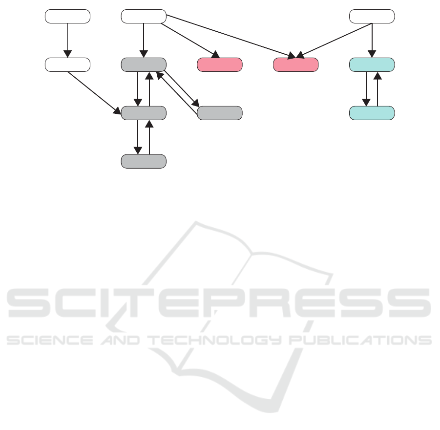
Figure 3: The State Transition Graph of star03.

Crafted Benchmark. We further contribute to an

artiﬁcial benchmark set named star to check the scal-

ability w.r.t. the number of automata, the number

of transitions, and the size of cyclic attractors. This

benchmark is available on the repository

Given a parameter N > 1, starN is an automata

network (Σ,S, T) deﬁned as follows.

• Σ = {a

| 1 ≤ i ≤ N}

• S = {a

} × {a

} × ·· · × {a

}

• T = {(a

,{a

| 1 ≤ j ≤ N,i ̸= j}) | 1 ≤ i ≤

N} ∪ {(a

,{}) | 1 ≤ i ≤ N}.

Each starN automata network contains N automata

that have two states, 2N transitions, and only one at-

tractor of size N + 1.

star03 is given below.

• Σ = {a

}

• S = {a

} × {a

}

• T = T

∪ T

– T

= {(a

,{a

}),(a

,{})}

– T

= {(a

,{a

}),(a

,{})}

– T

= {(a

,{a

}),(a

,{})}

Figure 3 shows the attractor of star03 in gray.

Bound k. For all benchmarks, the attractors are

known. In this experiment, we set a bound k for

each automata network so that solvers can compute

the largest attractors.

Environment. We execute all experiments on the

machine that equips 3GHz CPU and 16GB RAM. The

time limit is 3 hours.

6.2 Results

Table 3 shows comparisons between the proposed

method and the state-of-the-art existing ASP-based

method (Ben Abdallah et al., 2017). The ﬁrst col-

umn denotes the name of the automata networks. The

https://doi.org/10.5281/zenodo.7460387

BIOINFORMATICS 2023 - 14th International Conference on Bioinformatics Models, Methods and Algorithms

170

Table 3: Comparisons between Proposed SAT-based Methods and the Existing Method.

Statictics Proposed Existing

Instance |Σ| |T| Attractors k |S

max

| Basic +C +S +C+S ASP

Example 4 12 1(3):2(1):4(1) 4 3 1.6 1.6 1.7 1.7 0.2

Lambda phage 4 46 1(1):2(1) 2 4 1.7 1.8 1.8 1.7 0.1

Trp-reg 4 14 1(2):4(1) 4 3 1.7 1.7 1.7 1.7 0.2

Fission-yeast 9 43 1(1) 1 3 1.4 1.4 1.5 1.4 <0.1

Mamm. 10 34 1(1) 1 2 1.3 1.3 1.3 1.3 <0.1

Tcrsig 40 85 1(8) 1 2 1.6 1.7 1.8 1.8 <0.1

FGF 59 102 1(1536) 1 3 1.8 1.8 1.9 1.8 <0.1

T-helper 101 316 1(5875504) 1 3 88.6 86.6 88.9 88.4 148.3

star02 2 4 3(1) 3 2 1.3 1.3 1.3 1.3 0.1

star03 3 6 4(1) 4 2 1.4 1.5 1.3 1.5 0.3

star04 4 8 5(1) 5 2 1.7 1.6 1.6 1.6 0.6

star05 5 10 6(1) 6 2 2.0 1.9 1.7 1.8 1.6

star06 6 12 7(1) 7 2 2.6 2.2 2.1 2.1 3.6

star07 7 14 8(1) 8 2 6.5 2.8 2.4 2.3 10.7

star08 8 16 9(1) 9 2 46.5 5.9 2.9 2.7 27.1

star09 9 18 10(1) 10 2 538.6 36.7 3.4 3.2 65.2

star10 10 20 11(1) 11 2 6598.8 442.7 4.1 4.0 148.0

star11 11 22 12(1) 12 2 T.O. 8787.0 4.6 4.6 1088.2

star12 12 24 13(1) 13 2 T.O. T.O. 5.9 4.8 9959.3

star13 13 26 14(1) 14 2 T.O. T.O. 7.8 5.2 T.O.

star14 14 28 15(1) 15 2 T.O. T.O. 12.1 5.9 T.O.

star15 15 30 16(1) 16 2 T.O. T.O. 19.8 7.6 T.O.

star16 16 32 17(1) 17 2 T.O. T.O. 24.5 9.7 T.O.

star17 17 34 18(1) 18 2 T.O. T.O. 38.8 11.5 T.O.

star18 18 36 19(1) 19 2 T.O. T.O. 57.7 14.5 T.O.

star19 19 38 20(1) 20 2 T.O. T.O. 87.7 19.3 T.O.

star20 20 40 21(1) 21 2 T.O. T.O. 146.3 28.5 T.O.

star30 30 60 31(1) 31 2 T.O. T.O. 6250.3 614.4 T.O.

star40 40 80 41(1) 41 2 T.O. T.O. T.O. 7296.7 T.O.

second column denotes the number of automata in-

cluded. The third column denotes the number of

transitions included. The fourth column denotes the

sizes of the attractors. The number of attractors for

each size is displayed between the parenthesis. The

ﬁfth column denotes the bound k given to the solvers.

The sixth column denotes the maximum number of

states of automata denoted as S

max

. The seventh

to tenth columns denote the CPU time of the pro-

posed method. “Basic” denotes the basic constraint

model described in Section 3.2 with at least one con-

straint in Section 4.1. “+C” denotes the basic con-

straint model with the cycle constraint discussed in

Section 4.2. “+S” denotes the basic constraint model

with the symmetry breaking constraint discussed in

Section 4.3. “+C+S” denotes all constraints described

in Section 3.2 and Section 4. The eleventh col-

umn denotes the CPU time of the existing ASP-based

method.

In the biologically inspired benchmarks, all meth-

ods solved them within a few seconds. The main

reason is that they contain small-sized attractors and

thus k is also small. The difference between the pro-

posed methods and the ASP-based method mainly

comes from the implementation language: C++ and

Scala. The proposed method is implemented on Scala

which is running on a Java Virtual Machine (JVM) for

the modeling part and thus there is a small disadvan-

tage on this point. One exception is T-helper which

contains a large number of attractors. On this prob-

lem, our approach takes advantage of the SAT solver

BDD_MINISAT_ALL dedicated to the fast enumeration

of solutions.

On star benchmarks, the difference between each

method is more obvious. The CPU time of the ASP-

based method increases exponentially, and it cannot

solve star13 within 3 hours. On the other hand, al-

though “Basic” cannot solve star11, the two optional

constraints successfully improve “Basic”. The best

results are obtained by combining those constraints.

SAT-Based Method for Finding Attractors in Asynchronous Multi-Valued Networks

171

7 CONCLUSIONS

This paper describes a SAT-based method for ﬁnding

attractors of bounded size in asynchronous automata

networks. Attractors are crucial to validate the ini-

tial design of a biological model and predict possi-

ble asymptotic behaviors, e.g., how cells may result

through maturation in differentiated cell types. Given

a bound k, we propose a constraint model of trap do-

mains and compute attractors by incrementally com-

puting them from 1 to k. We further propose two op-

tional kinds of constraints to improve the computation

time of our approach. The ﬁrst one denotes cycle con-

straints which utilize a property of transitions in au-

tomata networks. The second one denotes symmetry

breaking constraints which reduce redundant search

spaces contained in the initial constraint model. Ex-

perimental evaluations are carried out over 30 au-

tomata networks. While the proposed SAT-based ap-

proach and the state-of-the-art ASP one could hardly

be discriminated on the few existing biologically in-

spired benchmarks, their behavior is quite different on

the crafted benchmarks we contribute. While the per-

formance of the initial SAT-based model is not so ef-

fective, adding optional constraints allows it to scale

much better than the ASP approach on benchmarks

with controlled attractor size. Future work is listed

as follows. Extending the comparisons to methods

of other networks like Boolean network (Mori and

Akutsu, 2022; Trinh et al., 2022; Rozum et al., 2021;

Inoue, 2011) is necessary. Extending the proposed

method to more complex networks like Petri net is

interesting. Supplementary materials of this paper is

available on the repository

ACKNOWLEDGEMENTS

This work was ﬁnancially supported by the “PHC

Sakura” program (43009SC, JPJSBP120193213), im-

plemented by the French Ministry for Europe and

Foreign Affairs, the French Ministry of Higher Ed-

ucation, Research and Innovation and the Japan So-

ciety for Promotion of Science. This work was

also supported by JSPS KAKENHI Grant Numbers

JP20K11748 and JP20H05794.

REFERENCES

Abou-Jaoudé, W., Monteiro, P. T., Naldi, A., Grandclaudon,

M., Soumelis, V., Chaouiya, C., and Thieffry, D.

https://doi.org/10.5281/zenodo.7460387

(2015). Model checking to assess t-helper cell plas-

ticity. Frontiers in bioengineering and biotechnology,

2:86.

Ben Abdallah, E., Folschette, M., Roux, O., and Magnin,

M. (2017). Asp-based method for the enumeration

of attractors in non-deterministic synchronous and

asynchronous multi-valued networks. Algorithms for

Molecular Biology, 12(1):1–23.

Biere, A., Fazekas, K., Fleury, M., and Heisinger, M.

(2020). CaDiCaL, Kissat, Paracooba, Plingeling and

Treengeling entering the SAT Competition 2020. In

Balyo, T., Froleyks, N., Heule, M., Iser, M., Järvisalo,

M., and Suda, M., editors, Proc. of SAT Competition

2020 – Solver and Benchmark Descriptions, volume

B-2020-1 of Department of Computer Science Report

Series B, pages 51–53. University of Helsinki.

Biere, A., Heule, M., van Maaren, H., and Walsh, T., editors

(2021). Handbook of Satisﬁability - Second Edition,

volume 336 of Frontiers in Artiﬁcial Intelligence and

Applications. IOS Press.

Chai, X., Ribeiro, T., Magnin, M., Roux, O., and Inoue,

K. (2020). Static analysis and stochastic search for

reachability problem. Electronic Notes in Theoretical

Computer Science, 350:139–158.

Crawford, J. M. and Baker, A. B. (1994). Experimental

results on the application of satisﬁability algorithms

to scheduling problems. In Proceedings of the 12th

National Conference on Artiﬁcial Intelligence (AAAI

1994), pages 1092–1097.

Crawford, J. M., Ginsberg, M. L., Luks, E. M., and

Roy, A. (1996). Symmetry-breaking predicates for

search problems. In Aiello, L. C., Doyle, J., and

Shapiro, S. C., editors, Proceedings of the Fifth Inter-

national Conference on Principles of Knowledge Rep-

resentation and Reasoning (KR’96), Cambridge, Mas-

sachusetts, USA, November 5-8, 1996, pages 148–

159. Morgan Kaufmann.

Davidich, M. I. and Bornholdt, S. (2008). Boolean network

model predicts cell cycle sequence of ﬁssion yeast.

PloS one, 3(2):e1672.

de Kleer, J. (1989). A comparison of ATMS and CSP tech-

niques. In Proceedings of the 11th International Joint

Conference on Artiﬁcial Intelligence (IJCAI 1989),

pages 290–296.

Fauré, A., Naldi, A., Chaouiya, C., and Thieffry, D. (2006).

Dynamical analysis of a generic boolean model for the

control of the mammalian cell cycle. Bioinformatics,

22(14):e124–e131.

Fitime, L. F., Roux, O., Guziolowski, C., and Paulevé,

L. (2017). Identiﬁcation of bifurcation transitions

in biological regulatory networks using Answer-Set

Programming. Algorithms for Molecular Biology,

12(1):19.

Folschette, M., Paulevé, L., Magnin, M., and Roux, O.

(2015). Sufﬁcient conditions for reachability in au-

tomata networks with priorities. Theoretical Com-

puter Science, 608:66–83.

Garg, A., Di Cara, A., Xenarios, I., Mendoza, L., and

De Micheli, G. (2008). Synchronous versus asyn-

chronous modeling of gene regulatory networks.

Bioinformatics, 24(17):1917–1925.

BIOINFORMATICS 2023 - 14th International Conference on Bioinformatics Models, Methods and Algorithms

172

Gebser, M., Kaminski, R., Kaufmann, B., and Schaub, T.

(2012). Answer Set Solving in Practice. Synthe-

sis Lectures on Artiﬁcial Intelligence and Machine

Learning. Morgan & Claypool Publishers.

Gelder, A. V. (2008). Another look at graph coloring via

propositional satisﬁability. Discrete Applied Mathe-

matics, 156(2):230–243.

Gershenson, C. (2002). Classiﬁcation of random boolean

networks. In Proceedings of the Eighth International

Conference on Artiﬁcial Life, pages 1–8.

Grieco, L., Calzone, L., Bernard-Pierrot, I., Radvanyi, F.,

Kahn-Perles, B., and Thieffry, D. (2013). Integrative

modelling of the inﬂuence of mapk network on can-

cer cell fate decision. PLoS computational biology,

9(10):e1003286.

Huang, S., Eichler, G., Bar-Yam, Y., and Ingber, D. E.

(2005). Cell fates as high-dimensional attractor states

of a complex gene regulatory network. Physical re-

view letters, 94(12):128701.

Inoue, K. (2011). Logic programming for boolean net-

works. In IJCAI 2011, Proceedings of the 22nd In-

ternational Joint Conference on Artiﬁcial Intelligence,

Barcelona, Catalonia, Spain, July 16-22, 2011, pages

924–930.

Iwama, K. and Miyazaki, S. (1994). SAT-variable complex-

ity of hard combinatorial problems. In Proceedings of

the IFIP 13th World Computer Congress, pages 253–

258.

Kauffman, S. A. (1969). Metabolic stability and epigene-

sis in randomly constructed genetic nets. Journal of

Theoretical Biology, 22(3):437–467.

Khaled, T. and Benhamou, B. (2020). An asp-based ap-

proach for boolean networks representation and at-

tractor detection. In LPAR, pages 317–333.

Klamt, S., Saez-Rodriguez, J., Lindquist, J., Simeoni, L.,

and Gilles, E. (2006). A methodology for the struc-

tural and functional analysis of signaling and regula-

tory networks. BMC Bioinformatics, 7(1):56.

Levy, N., Naldi, A., Hernandez, C., Stoll, G., Thieffry, D.,

Zinovyev, A., Calzone, L., and Paulevé, L. (2018).

Prediction of Mutations to Control Pathways Enabling

Tumour Cell Invasion with the CoLoMoTo Interactive

Notebook (Tutorial) . Frontiers in Physiology, 9:787.

Mbodj, A., Junion, G., Brun, C., Furlong, E. E., and Thief-

fry, D. (2013). Logical modelling of drosophila sig-

nalling pathways. Molecular BioSystems, 9(9):2248–

2258.

Mori, T. and Akutsu, T. (2022). Mini review attractor de-

tection and enumeration algorithms for boolean net-

works. Computational and Structural Biotechnology

Journal.

Naldi, A., Hernandez, C., Levy, N., Stoll, G., Monteiro,

P. T., Chaouiya, C., Helikar, T., Zinovyev, A., Cal-

zone, L., Cohen-Boulakia, S., et al. (2018). The

colomoto interactive notebook: accessible and repro-

ducible computational analyses for qualitative biolog-

ical networks. Frontiers in physiology, 9:680.

Paulevé, L. (2016a). Goal-oriented reduction of automata

networks. In International Conference on Compu-

tational Methods in Systems Biology, volume 9859

of Lecture Notes in Bioinformatics, pages 252–272.

Springer.

Paulevé, L. (2016b). Goal-oriented reduction of automata

networks. In International Conference on Computa-

tional Methods in Systems Biology, pages 252–272.

Springer.

Paulevé, L. (2017). Pint: a static analyzer for transient

dynamics of qualitative networks with IPython inter-

face. In CMSB 2017 - 15th conference on Computa-

tional Methods for Systems Biology, volume 10545 of

Lecture Notes in Computer Science, pages 309–316.

Springer International Publishing.

Paulevé, L., Andrieux, G., and Koeppl, H. (2013). Under-

approximating cut sets for reachability in large scale

automata networks. In International Conference on

Computer Aided Veriﬁcation, pages 69–84. Springer.

Paulevé, L., Magnin, M., and Roux, O. (2012). From the

Process Hitting to Petri Nets and Back. Technical Re-

port hal-00744807, ETH Zürich.

Rougny, A., Paulevé, L., Teboul, M., and Delaunay, F.

(2021). A detailed map of coupled circadian clock and

cell cycle with qualitative dynamics validation. BMC

bioinformatics, 22(1):1–24.

Rozum, J. C., Deritei, D., Park, K. H., Gómez Tejeda Za-

ñudo, J., and Albert, R. (2021). pystablemotifs:

Python library for attractor identiﬁcation and control

in Boolean networks. Bioinformatics, 38(5):1465–

1466.

Sahin, Ö., Fröhlich, H., Löbke, C., Korf, U., Burmester,

S., Majety, M., Mattern, J., Schupp, I., Chaouiya, C.,

Thieffry, D., et al. (2009). Modeling erbb receptor-

regulated g1/s transition to ﬁnd novel targets for de

novo trastuzumab resistance. BMC systems biology,

3(1):1–20.

Simão, E., Remy, E., Thieffry, D., and Chaouiya, C. (2005).

Qualitative modelling of regulated metabolic path-

ways: application to the tryptophan biosynthesis in e.

coli. Bioinformatics, 21(suppl 2):ii190–ii196.

Soh, T., Banbara, M., and Tamura, N. (2017). Proposal and

evaluation of hybrid encoding of CSP to SAT integrat-

ing order and log encodings. International Journal on

Artiﬁcial Intelligence Tools, 26(1):1–29.

Tamura, N., Taga, A., Kitagawa, S., and Banbara, M.

(2009). Compiling ﬁnite linear CSP into SAT. Con-

straints, 14(2):254–272.

Thieffry, D. and Thomas, R. (1995). Dynamical behaviour

of biological regulatory networks—ii. immunity con-

trol in bacteriophage lambda. Bulletin of Mathemati-

cal Biology, 57(2):277–297.

Thomas, R. (1973). Boolean formalization of genetic

control circuits. Journal of Theoretical Biology,

42(3):563 – 585.

Toda, T. and Soh, T. (2016). Implementing efﬁcient all

solutions SAT solvers. ACM J. Exp. Algorithmics,

21(1):1.12:1–1.12:44.

Trinh, V.-G., Hiraishi, K., and Benhamou, B. (2022). Com-

puting attractors of large-scale asynchronous boolean

networks using minimal trap spaces. In Proceedings

of the 13th ACM International Conference on Bioin-

SAT-Based Method for Finding Attractors in Asynchronous Multi-Valued Networks

173

formatics, Computational Biology and Health Infor-

matics, pages 1–10.

Tseitin, G. S. (1968). On the complexity of derivations

in the propositional calculus. Studies in Mathematics

and Mathematical Logic Part II, pages 115—-125.

Walsh, T. (2000). SAT v CSP. In Proceedings of the 6th

International Conference on Principles and Practice

of Constraint Programming (CP 2000), pages 441–

456.

Wuensche, A. (1998). Genomic regulation modeled as a

network with basins of attraction. In Paciﬁc Sympo-

sium on Biocomputing, volume 3, pages 89–102.

BIOINFORMATICS 2023 - 14th International Conference on Bioinformatics Models, Methods and Algorithms

174