Dense Point-to-Point Correspondences Between Genus-Zero Shapes

Using Cubic Mapping and Horn-Schunck Optical Flow

Pejman Hashemibakhtiar

1,2

, Thierry Cresson

1,2

, Jacques De Guise

1,2

and Carlos Vázquez

1,2

Département de Génie Logiciel et TI, École de Technologie Supérieure (ÉTS), Montréal, Canada

Laboratoire de Recherche en Imagerie et Orthopédie (LIO), Centre de Recherche du CHUM, Montréal, Canada

Keywords: Dense Correspondence Map Computation, Computational Geometry, non-Rigid non-Isometric Deformation,

Cubic Mapping, Optical Flow.

Abstract: Establishing correspondences is a fundamental and essential task in computer graphics for further

processing of shapes. We have proposed an important modification to an existing method to remove several

large matching errors in specific regions. The method uses the unit sphere and the regular spherical grid as

parameterization spaces to perform registration and obtain the matching map between two three-

dimensional genus-zero shapes, considering non-rigid and non-isometric deformations. Although the unit

sphere is a suitable parameterization space for rigid alignment, mapping the sphere to a regular spherical

grid for non-rigid registration makes the process unstable since it is not a distance-preserving projection.

Therefore, it produces large detachments on the grid and for several regions. Replacing the regular spherical

grid mapping with Cubic mapping results in smooth displacement and locality for all corresponding vertices

on each cube face. Due to our enhancement, the Optical Flow faces a smooth flow field in the non-rigid

registration process. Our modification results in the elimination of matches with significant normalized

geodesic error and an increase in the accuracy of the correspondence map, compared to the base method and

other recently published approaches.

1 INTRODUCTION

Finding the correspondence map between two

meshes is an essential initializing task for further

processing of the shapes, such as building a

Statistical Shape Model (SSM), Shape

Reconstruction, Shape Analysis, etc. (Sahillioğlu,

2019). For building an SSM of the shape of interest,

correspondences should be established for all shapes

within the dataset (Cootes et al., 1995), and to have

an accurate SSM, we need to establish correct

correspondences (Davies et al., 2002). Thus,

matching errors on the correspondence map should

be removed or decreased. If the matched vertices do

not represent anatomically equivalent regions on

source and target shapes (e.g., matching the left foot

to the right foot in matching human shapes as

depicted in Figure 1a), the result of the SSM and its

variability will be exaggerated (Davies et al., 2002),

leading the application toward unexpected results.

The task becomes more complex as shapes go from

2D to 3D, and the transformation goes from rigid to

non-rigid and from isometric to non-isometric

(Sahillioğlu, 2019). In addition, it is a challenging

process since shapes’ local and global information

should be considered (Sahillioğlu, 2019). Since most

real shapes tend to have non-rigid and non-isometric

deformations, matching such shapes has become an

interesting and expanding topic in computer vision.

Multiple surveys represent recent advances in

establishing correspondences (Sahillioğlu, 2019; Li

et al., 2014; Tam et al., 2012). The author

(Sahillioğlu, 2019) has presented a classification of

recent methods based on the density of the

Figure 1: (a) Several erroneous matchings in a region by a

matching algorithm (Lee et al., 2019); (b) ground truth.

196

Hashemibakhtiar, P., Cresson, T., De Guise, J. and Vázquez, C.

Dense Point-to-Point Correspondences Between Genus-Zero Shapes Using Cubic Mapping and Horn-Schunck Optical Flow.

DOI: 10.5220/0011674900003417

In Proceedings of the 18th International Joint Conference on Computer Vision, Imaging and Computer Graphics Theory and Applications (VISIGRAPP 2023) - Volume 1: GRAPP, pages

196-205

ISBN: 978-989-758-634-7; ISSN: 2184-4321

 2023 by SCITEPRESS – Science and Technology Publications, Lda. Under CC license (CC BY-NC-ND 4.0)

correspondences, deformation types, solution

approaches, etc. Regarding the solution approaches,

the first category is Similarity-based solutions

(Ovsjanikov et al., 2012; Nogneng et al., 2017; Ren

et al., 2018; Gehre et al., 2018; Melzi et al., 2018;

Hu et al., 2021; Vestner et al., 2017) in which

geometric invariants descriptors are computed and

matched. These sophisticated descriptors need to

handle different geometric aspects of the shapes,

e.g., rigid alignments, scaling, etc. The other

approaches are Registration-based methods

(Eisenberger et al., 2020; Eisenberger et al., 2019;

Cosmo et al., 2019; Dyke et al., 2019; Melzi et al.,

2019; Lee et al., 2019). These techniques register

shapes under a deformation field or project them

into a common intermediate domain and perform the

registration in the parameterization space. The

significant advantage of these approaches is that

they generate one-to-one, very dense, and

continuous correspondence maps (Huang et al.,

2020). Although parametrizing the shapes, results in

higher computational complexity than similarity-

based methods (Sahillioğlu, 2019), it can help tackle

some challenges in parametrization spaces.

Removing the scale of shapes by mapping them to

unit disks (Sahillioğlu, 2019), handling the rigid

registration easier by mapping shapes into spheres

(Lee et al., 2019), using intrinsic and extrinsic

information to handle local and global deformations

(Eisenberger et al., 2020) and matching the shapes

using functional maps (Melzi et al., 2018) are

examples of parameterization done in the literature.

(Eisenberger et al., 2020) use an intermediate

product space that includes shapes’ intrinsic and

extrinsic information and perform the registration

process fused with functional maps. Intrinsic

information is invariant to large-scale deformations,

and extrinsic features handle local topological

changes. So, rigid alignment is implicitly

considered. Although they have suggested that their

initial pose determination using Markov Chain

Monté Carlo provides reasonable estimation in many

cases, the results show that initialization still can go

wrong for large deformations, affecting the matching

results. (Eisenberger et al., 2019) utilize the

Karhunen-Loéve expansion to compute divergence-

free deformation fields. This property makes the

registration applicable to shapes with almost the

same volume, which is a drawback for a general

matching algorithm. (Cosmo et al., 2019) have used

the Laplacian spectrum to deform shapes. The

method works on shapes from different categories

(e.g., matching horses to camels) having the same

initial pose only. (Dyke et al., 2019) add anisotropic

deformations to a non-rigid registration process to

handle the non-isometric deformations accurately.

Although they handle large-scale deformations, the

initialization of the method is based on their local

feature descriptor, and poor initial matches mislead

the registration process entirely. In (Melzi et al.,

2019), iterative up-sampling is used in the spectral

domain to refine the functional map results. The

functional map initialization implicitly considers the

shapes’ initial pose. Unit spheres and regular

spherical grids are incorporated to match two genus-

zero shapes (Lee et al., 2019). Learning-based

approaches are also used for finding the

correspondences on shapes. However, they take

longer processing time in the training stage rather

than processing the shapes directly (Sahillioğlu,

2019) and need the availability of large datasets.

For building an SSM, it is critical that the

corresponding landmarks are sufficiently dense and

smoothly continuous (Munsell et al., 2008). As

stated, registration-based methods represent dense

and continuous correspondences on shapes (Huang

et al., 2020).

(Lee et al., 2019) have used the unit sphere as the

intermediate domain since it is a suitable

parameterization space for explicitly handling scale

and rigid transformation. In addition, significant

differences in the initial pose can be handled on the

unit sphere. Figure 2 elaborates steps of their

framework resulting in matching between two cat

shapes (Figure 2a). First, shapes are converted into

unit spheres (Figure 2b) using Conformalized Mean

Curvature Flow (CMCF) (Kazhdan et al., 2012).

Spheres are then processed by Authalic Evolution

(AE) (Zou et al., 2011) to make the area of the mesh

triangles as equal as possible (Figure 2c). Heat

Kernel Signature (HKS) (Sun et al., 2009) is

calculated on the shape domain and is pulled back to

the sphere (Figure 2d). It extracts features of the

shapes that are used in rigid and non-rigid

registration steps. Rotational alignment is applied

(Figure 2e) to align the spheres as much as possible

by maximizing the correlation on SO(3) (Baden et

al., 2018). Finally, for the non-rigid registration step,

the spheres are moved into an equirectangular

spherical grid (Figure 2f) with multiple resolutions,

simulating the hierarchy structure of the Optical

Flow process (Prada et al., 2016). After applying the

Optical Flow on hierarchical planar grids, the flow

field is pulled back into spheres, and vertices of the

source sphere are moved to their corresponding

coordinates on the target sphere accordingly (Figure

2g). Calculating a proximity metric on overlapped

spheres, e.g., Euclidean distance, generates the

Dense Point-to-Point Correspondences Between Genus-Zero Shapes Using Cubic Mapping and Horn-Schunck Optical Flow

197

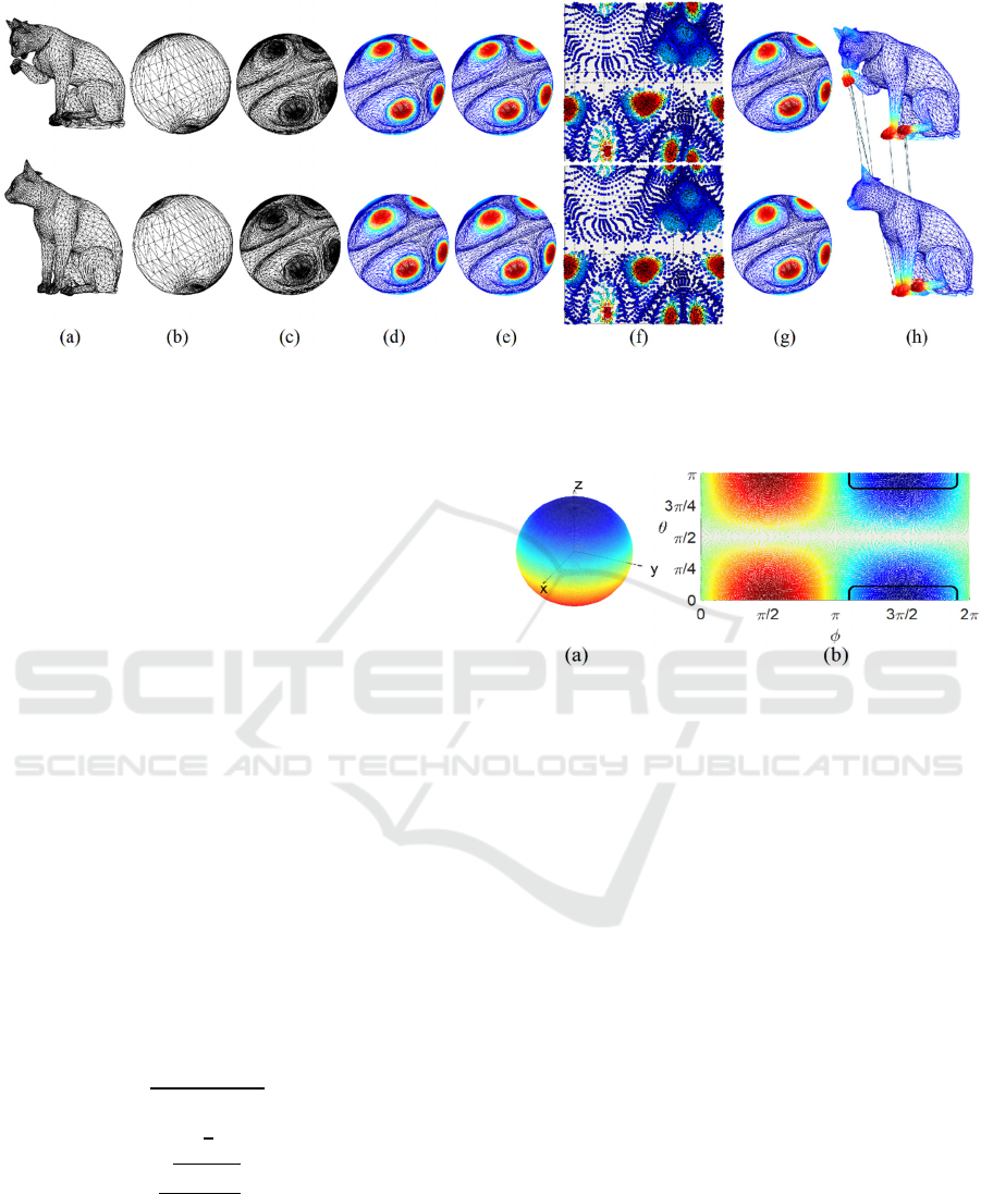
Figure 2: Illustration of (Lee et al., 2019) work. (a) Source (top) and target (bottom) cat shapes; (b) Shapes are moved into

the spherical domain; (c) AE method applied; (d) HKS is computed on the shape domain and pulled back on the spheres; (e)

Spheres are rotationally aligned; (f) Spheres are moved to a regular equirectangular spherical grid; (g) Non-rigid registration

is applied using Optical Flow on grids and spheres are advected; (h) Proximity measure reveals the matching of vertices.

forward and backward correspondence maps (Figure

2h). However, looking at the result of the method,

we can figure out that several erroneous matchings

are represented in some areas (e.g., Figure 1a),

which will be investigated in the next section.

2 PROBLEM STATEMENT

In (Lee et al., 2019), authors have stated that they

“rasterize the scale factors from the spherical

triangulation” (Figure 2e) “onto an equirectangular

N×N spherical grid” (Figure 2f) to perform Authalic

Evolution. They have used the same approach for

the Optical Flow process, stating that the

computation of the flow field is done “using regular

N×N spherical grids and rasterizing the signals”,

HKS

and T

HKS

the HKS signals defined on the

source and target shapes.

As defined in the standard ISO 31-11, the

parameterization from a sphere in cartesian space

(Figure 3a) to a regular spherical grid (Figure 3b) is

done by the following formulas.

ρ =









z



; ρ0

=arctan





;0

π

φ = arctan



√



z





;0φ2π

(1)

On a unit sphere, ρ is equal to 1. Thus, the

parameters θ and φ reconstruct the UV plane (Figure

3b). However, this parametrization is not distance-

preserving for vertices that have border values of θ

Figure 3: Illustration of parameterization from a unit

sphere (a) to a regular spherical grid (b). The mapping has

not preserved the distances as they are on the sphere. The

indicated region is an example of the issue.

(close to 0 or π) and φ (close to 0 or 2π), which we

will refer to as “border vertices”. Although these

vertices are located very close in the spherical

domain (e.g., dark blue regions on top of the sphere

in Figure 3a), they are far apart on the UV plane

(indicated dark blues regions on top and bottom of

the rectangular grid in Figure 3b). (Lee et al., 2019)

move two rigidly aligned spheres into spherical grids

(Figure 2e to 2f), and then, the Optical Flow will

As two spheres are rigidly registered, the

corresponding vertices are close in the spherical

domain, and some small and smooth movements

should match them. However, a slight shift of the

border vertices in the spherical domain can be

mapped to a significant shift on the UV grid. E.g., a

slight movement of vertices in the dark blue region

of Figure 3a can move the vertex from the upper

region indicated in Figure 3b to the bottom one.

With the Optical Flow operating on this planar

domain, it cannot recover these large shifts and will

GRAPP 2023 - 18th International Conference on Computer Graphics Theory and Applications

198

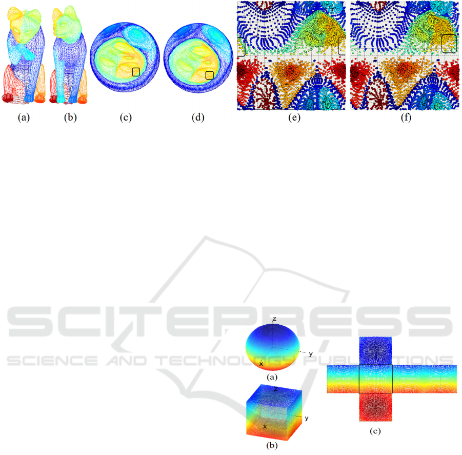
Figure 4: Illustration of discontinuity of neighbor regions on the spheres when they are projected to the spherical grid; (a)

Source shape; (b) Target shape; (c) Source sphere rigidly registered into target sphere. The region which will be split when

mapping into the spherical grid is indicated; (d) Target sphere. Corresponding region is indicated; (e) Spherical grid

representation of the source sphere indicating the region that is splitting into two regions, dissimilar to its correspondence

region in target grid representation; (f) Spherical grid representation of the target sphere, showing the corresponding region

to the indicated region in the source grid while it is a single connected area on the right side of the grid.

fail to match those corresponding vertices.

An illustration of this problem is represented in

Figure 4. Figure 4a is the source cat shape which

will be put in correspondence with the target cat

shape, represented in Figure 4b. The coloring

represents corresponding landmarks on both shapes.

Figures 4c and 4d show rigidly aligned spherical

representations of the two shapes and indicate the

regions containing some border vertices, which will

be investigated further on their planar representation.

The spherical grid parameterization of the shapes in

Figures 4e and 4f implies that although most of the

vertices in the indicated regions are in the same

location on the spherical grid, some vertices of one

of the cat’s ears are separated on the source planar

representation (as indicated in Figure 4e), while they

are all located on the right side of the plane in the

target planar representation (Figure 4f). Since

corresponding vertices are placed far from each

other in the planar domain, the Optical Flow cannot

find proper movement for matching these vertices.

3 METHODOLOGY

To solve the issue of border vertices, we propose

replacing the regular spherical mapping (steps in

Figure 2e and 2f) with cubic mapping (Greene,

1986). Figure 5a shows a unit sphere with smooth

coloring on its surface. Moving the sphere to a unit

cube (Figure 5b) and expanding it (Figure 5c) shows

that on each face, the distances and locality are

preserved (according to the fact that colors are not

distorted as we saw in Figure 3b for the regular

spherical grid).

To avoid the spherical grid mapping issue

(having large displacements) for some vertices on

the expanded version of the unit cube, we extended

each face of the cube properly while respecting the

adjacency of the faces and the locality of the vertices

on the cube. For applying the Optical Flow, we only

consider the central face (indicated in Figure 5c with

a black rectangle). By doing this for all six faces

separately, we can have a continuous, local, and

smooth flow field for all the vertices.

Figure 5: Replacing the regular spherical grid with cubic

mapping. (a) The unit sphere; (b) The unit cube made by

cubic mapping from the unit sphere; (c) cubic mapping

expanded. The expansion is done according to the central

indicated face and adjacent faces.

Figure 6 shows the expanded cube for the cat

shape represented in Figure 4a. The indicated region

in Figure 6 implies that the vertices of the cat’s ear

are all connected in the same region, while they have

been split in the previous parameterization (Figure

4e). This shows that the central face of the expanded

version of the cube keeps all adjacent vertices in a

single connected region.

The mentioned modification is explained in

detail in Algorithm 1, which will replace the

Dense Point-to-Point Correspondences Between Genus-Zero Shapes Using Cubic Mapping and Horn-Schunck Optical Flow

199

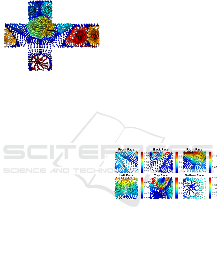
Figure 6: Cubic mapping expanded for cat shape

represented in Figure 4. The indicated part is the ear of the

cat, which is split into two regions in Figure 4e.

Algorithm 1: Proposed modification to (Lee et al., 2019)

by incorporating Cubic Mapping.

Input : Rotationally aligned Source and Targe

Spheres, S

Sphere

and T

Sphere

Output : Forward M

S→T

, and Backward M

T→S

Correspondence Maps

1 : For i=1:max

level

tical

flow

2 : res=level_resolutions(i)

3 : Compute cubes S

Cube

, T

Cube

from S

Sphere

respectively. faces will be

generated according to

image_generation_resolution, S

HKS(i+1)

and T

HKS(i+1)

4 : For j=1 to 6{front, back, right, left, top,

ottom

}

5 : Extend S

Cube_face(j)

, T

Cube_face(j)

according to their adjacent faces and

generate S

image(j)

, T

image(j)

6 : Interpolate S

image(j)

, T

image(j)

using

gaussian filter to fill the holes on the

ima

7 : Reduce the image resolutions to res

8 : Apply Optical Flow on S

image(j)

and keep the calculated flow

field for the face S

Cube_face(j)

9 : For j=1 to 6{front, back, right, left, top,

ottom

}

10 : Move the vertices falling on

Cube_face(j)

and update S

Sphere

accordingl

11 : Compute M

S→T

, and M

T→S

using the

roximit

non-rigid registration part in (Lee et al., 2019). After

aligning two spheres rigidly, the spheres are

transferred into unit cubes (Algorithm 1, line 3).

Each face will be appropriately extended with its

adjacent faces on the cube, and the Optical Flow is

applied to it (Algorithm 1, lines 4 to 8). Finally, the

computed flow field for all vertices is pulled back to

the source sphere and they are advected accordingly.

To prove that the locality is preserved for this

parametrization, we move two rigidly registered

spheres with known correspondences into unit cubes

(Algorithm 1, line 3) and then overlay the

corresponding faces of the cubes to compute the

Euclidean distances from each vertex on the source

cube face to its corresponding vertex on the target

cube face. Assuming that the corresponding vertices

are close on the overlaid spheres (since spheres have

been rigidly registered), corresponding vertices on

the source cube and target cube can be located on

the same face (e.g., both on front faces of cubes), or

adjacent faces (top, bottom, left and right faces for

the front face). Considering this adjacency, Figure 7

shows the Euclidean distances for vertices on the

source cube faces to their corresponding vertices on

the overlaid target cube faces. The cube is unit, and

the displacement of all vertices is less than half of

the side of each face. The distances can differ due to

the amount of deformation of the shapes.

We replaced the non-rigid registration process in

(Lee et al., 2019) with Algorithm 1. We will show

that our approach has resolved the mentioned issue

in (Lee et al., 2019) in multiple datasets and

according to multiple matching quality metrics.

Figure 7: Indicating Euclidean distance of the

corresponding vertices on the cube surfaces. The cube

faces are sized 1 by 1.

4 EXPERIMENTS AND RESULTS

Looking closely at the results of (Lee et al., 2019),

we figure out that the problem only occurs for some

border vertices. Depending on the amount of

deformation of the target shape with respect to the

source shape and rotational alignment of the spheres,

some of the border vertices might need large

displacements to meet the location of their

correspondences on the regular spherical grids.

Although there could be a small number of border

vertices having such a property, the wrong matching

of one vertex can also mislead the matching result

GRAPP 2023 - 18th International Conference on Computer Graphics Theory and Applications

200

for its neighbors since the registration process is

done locally by Optical Flow.

To analyze the result of the proposed

modification, matching accuracy for the border

vertices will be considered only. We define border

vertices as follows. After moving a sphere into the

regular spherical grid, vertices that fall into 10% of

the margins from the borders of θ and φ parameters

are stated as border vertices. The 10% value is set

experimentally and will ensure that all the probable

erroneous matchings are happening for vertices in

this set. Eq. 2 shows this criterion.

0



; π−



π

0φ

2π

; 2π−

2π

φ2π

(2)

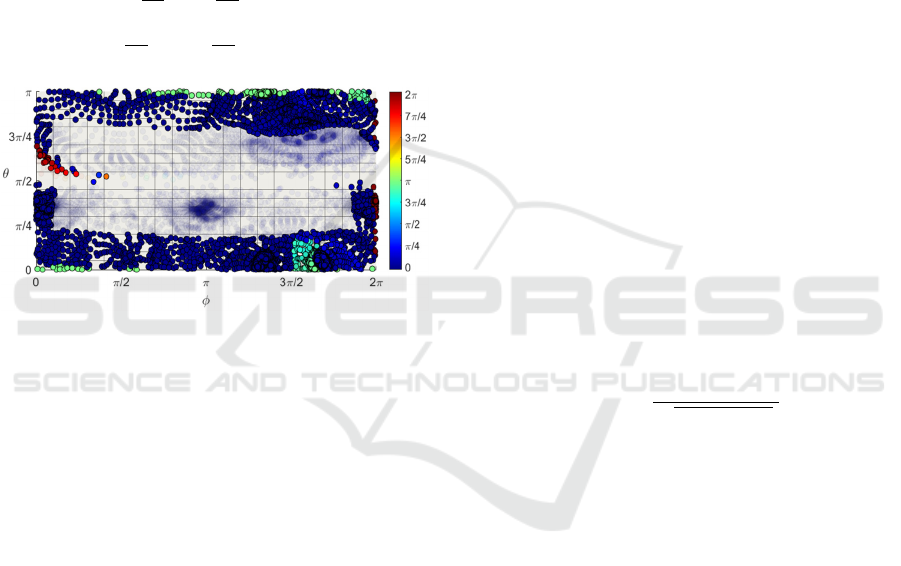
Figure 8: Indicating Euclidean distance for corresponding

vertices on the spherical grids. Non-border vertices are set

transparent. Large distances of some border vertices,

implying cases that cannot be matched with the Optical

Flow on this grid.

Figure 8 represents the Euclidean distance

between the vertices on the source spherical grid and

their corresponding vertices on the overlaid target

spherical grid for two shapes with known

correspondences. In the figure, border vertices

defined by Eq. 2 are shown as filled circles, while

non-border vertices are shown transparently.

According to the figure, although most of the border

vertices are very close to their corresponding

matches on the target grid (distances are close to 0),

some cases need to traverse to the other side of the

grid to be matched to their correspondences

(distances are close to π or 2π).

To demonstrate the effectiveness of the

modification applied to (Lee et al., 2019), we

considered comparing registration results from (Lee

et al., 2019) as ‘DenseP2PCorr’, the modified

version of the method by incorporating the cubic

mapping as ‘Ours’, ‘Zoom Out’ (Melzi et al., 2019)

and ‘Smooth Shells’ (Eisenberger et al., 2020) as

registration-based approaches. These methods result

in dense corresponding maps while handling rigid

alignment and obtaining the matching between

shapes with different poses. Three datasets are

considered in this experiment as they contain shapes

from the real world with non-rigid and non-isometric

deformations. TOSCA dataset (Bronstein et al.,

2008) consists of 80 models in 9 categories with

mesh resolutions ranging from 4K to 53K. Sumner

dataset (Sumner et al., 2004) consists of 76 non-

animative models in 8 categories with resolutions

ranging from 5K to 43K. The third database is

SCAPE (Anguelov et al., 2005), containing 72

models of human shape with a resolution of 12.5K

vertices. All shapes in all datasets are in

correspondence within each category and are

represented with the same topology, making them

suitable benchmarks for correspondence evaluation.

However, to reduce the time complexity of the

runtime, we considered a subset of the shapes for the

matching process. The number of combinations

within each category is represented in Table 1.

To evaluate the methods, we used Princeton

benchmark protocol and Correspondence Quality

Characteristics (CQC) curves (Kim et al., 2011).

Assume that a matching algorithm has matched

vertex x from source shape to vertex y in target

shape as (x,y). Having the ground truth of the match

as (x,y



), Normalized Geodesic Error (NGE) for

the match (x,y) is calculated by Eq. 3.

NGE(x,

dist



(



)



Shape_Area

(3)

In Eq. 3., dist



(y,y



) is the geodesic distance

calculated on the target mesh between vertices y and



, and Shape_Area is the sum of the surface areas

for the target shape. For optimizing the computation

complexity, dist



(y,y



) is calculated and stored

for all combinations of y and y



on each shape and

for all participating shapes within each dataset.

Since the modification of the algorithm affects

the border vertices, NGE for these vertices is

considered and averaged as the results in Table 1.

In addition to the numerical analysis in Table 1,

visual comparisons of matching results of (Lee et al.,

2019) vs. ours are represented in Figures 9-11.

Figure 9a shows a cat shape on the left, while it

shows its spherical grid representation on the right.

The coloring represents the vertex indices on the

shape and the spherical grid. Considering the same

coloring on the shape and grid, border vertices inside

the yellow rectangle represent the region on the cat’s

Dense Point-to-Point Correspondences Between Genus-Zero Shapes Using Cubic Mapping and Horn-Schunck Optical Flow

201

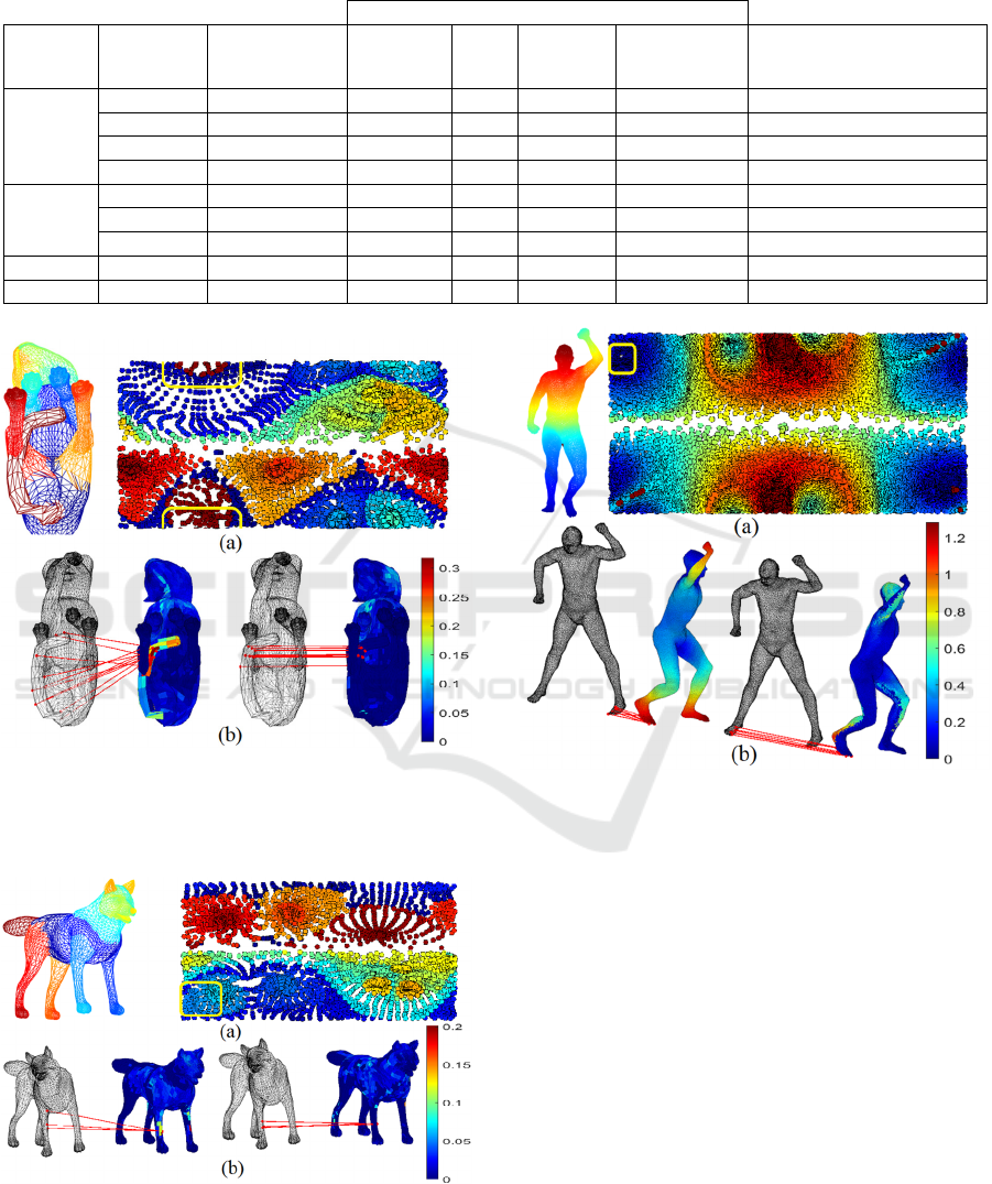
Table 1: Average Normalized Geodesic Error for border vertices and non-isometric deformation per category and in total

for all datasets.

Average NGE (×10

-3

)

Dataset/

Method

Shape

Category

Number of

Combinations

DenseP2

PCorr.

Ours

Smooth

Shells

Zoom Out NID average (×10-3)

TOSCA

Wolf 6 11.5 4.5 0.7 71.2 18.56

Centau

30 30.5 16.7 42.8 472 34.23

Horse 56 30.8 18.4 34.1 289.2 39.53

Total 142 30.3 17.6 35.9 338.2 37.59

Sumner

Lion 72 49.6 31.6 243.6 389 44.97

Cat 72 52.3 24.3 242.6 469.7 63.61

Total 144 51.4 26.8 242.9 441.8 55.98

SCAPE Human 110 107.2 25.9 62.2 80.6 39.4

Total Total 396 60.6 22.6 97.4 281.1 42.46

Figure 9: (a) Indicating some border vertices on the tail of

the cat; (b) Comparing the matching results from

DenseP2PCorr (left) vs. Ours (right) on two cat shapes in

the Sumner dataset.

Figure 10: Indicating some border vertices on the hand of

the wolf; (b) Comparing the matching results from

DenseP2PCorr (left) vs. Ours (right) on two wolf shapes in

the TOSCA dataset.

Figure 11: (a) Indicating some border vertices on the foot

of the human; (b) Comparing the matching results from

DenseP2PCorr (left) vs. Ours (right) on two human shapes

in the SCAPE dataset.

tail. Figure 9b shows the matching results by (Lee et

al., 2019) on the left and our approach on the right.

The coloring in Figure 9b represents the NGE of the

matching for all vertices in the shape domain. Figure

10 and Figure 11 show similar results for the

registration of two wolf shapes from the TOSCA

dataset and two human shapes from the SCAPE

dataset, respectively.

Furthermore, we have represented CQC curves

for all methods within each category in all datasets.

CQC curves (Kim et al., 2011) represent percentages

of correct matches that are tolerating distance r in

terms of NGE. Figure 12 shows all CQC curves for

each category within each dataset. In addition,

curves for all shapes within each dataset and all

GRAPP 2023 - 18th International Conference on Computer Graphics Theory and Applications

202

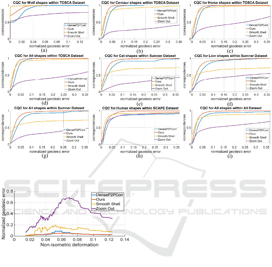
Figure 12: CQC curves for all datasets per category and in total. (a) Wolf shapes from TOSCA; (b) Centaur shapes from

TOSCA; (c) Horse shapes from TOSCA; (d) All shapes within TOSCA; (e) Cat shapes from Sumner; (f) Lion shapes from

Sumner; (g) All shapes within Sumner; (h) Human shapes from SCAPE; (i) All shaped within all datasets.

Figure 13: Normalized Geodesic Error (NGE) vs. non-

isometric deformation (NID) of shapes for all matching

results.

shapes within all datasets are also represented. The

border vertices on target spherical grids are

considered only for generation of CQC curves.

Finally, to demonstrate the amount of non-

isometric deformations of the shapes and how they

affect the result of different matching processes, we

define the Non-Isometric Deformation (NID) as

follows.

NID

(

)

=NGE

(

)





−NGE

(

)







(4)

The source and target shapes are arbitrary shapes

within the same category (having the same

topology), and x and y are all vertices on each shape.

This metric is calculated for all combinations of the

shapes participating in the matching experiment. The

values are averaged within each category and

represented in Table 1.

Taking the NID into account, we have

demonstrated the amount of NGE for the matching

result with respect to the NID of the matching

shapes for all four competing methods in Figure 13.

5 DISCUSSION AND

CONCLUSION

As stated in Table 1, almost 400 registration

processes are done to demonstrate the comparison of

the accuracy of corresponding maps generated by

four different methods in three different datasets

with different characteristics. Among all the

categories, the Wolf category from the TOSCA

dataset is the easiest matching case since shapes are

not deformed very much (as an example is

represented in Figure 10b), and the density of the

shapes is the lowest (approximately 4K vertices). In

addition, the initial states of the shapes are very

similar. On the contrary, the human shapes in the

Dense Point-to-Point Correspondences Between Genus-Zero Shapes Using Cubic Mapping and Horn-Schunck Optical Flow

203

SCAPE dataset have a broad range of initial poses

and deformations. As shown in Table 1, our

approach has reduced the NGE for border vertices,

making the matching results more accurate than

those from (Lee et al., 2019) among all categories. It

also represents better results compared to the other

two methods when the shapes’ NID increases. The

information on NID demonstrates the effect of the

nature of the shapes on the result of registration

processes. As can be seen, the shapes in the Wolf

category from TOSCA, which have the least NID

values, are best matched with the Smooth Shell

(Eisenberger et al., 2020) among the competitors.

Zoom Out (Melzi et al., 2019) is always resulting

less accurate matching than the others.

Visual comparisons in Figures 9-11 demonstrate

the erroneous matching result for some of the border

vertices in the result of (Lee et al., 2019) vs. Ours.

Figure 9a implies the same coloring for the cat shape

and the parameterized vertices on the spherical grid.

The vertices indicated in crimson color on the grid

show cat’s tail, as can be seen on the cat shape with

the identical coloring. It is depicted in Figure 9b that

these border vertices represent significant matching

errors, and they are chaotically matched from the

source shape to multiple regions on the target shape

by (Lee et al., 2019) (left). This behavior is removed

in the result of our proposed method (right). In

addition, we can see that only some border vertices

show significant errors, and almost all non-border

vertices are matched to their correct

correspondences correctly. Similar behavior is

shown for the Wolf shapes in Figure 10 and Human

shapes in Figure 11.

Figure 12 represents CQC curves for all shapes

within each category and dataset. As shown in

Figure 12a, the Smooth Shell (Eisenberger et al.,

2020) outperforms the others only when shapes are

not deforming non-isometrically very much (wolf

category of the TOSCA dataset). In addition, the

amount of improvement to the matching accuracy

among border vertices is related to the amount of

non-rigid deformation represented in the shapes and

the number of border vertices that are dislocated

with large distances on the spherical grid in the

approach represented by (Lee et al., 2019).

Considering the mentioned criteria, Figure 12b-12h

shows that our modification improved the accuracy

compared with (Lee et al., 2019) for all categories

and within all datasets. Figure 12i shows the results

of the comparison in all registration processes.

According to Figure 13, the more non-isometric

deformation a target shape (concerning the source

shape) has, the more challenging the registration

process is to match corresponding vertices. As stated

in the figure, the Smooth Shell method (Eisenberger

et al., 2020) can represent the best result of matching

for the shapes having small values of NID (e.g.,

Wolf category of the TOSCA dataset). However,

with increasing the NID of the registering shapes,

the Smooth Shell’s NGE increases compared to Ours

and DenseP2PCorr. The fluctuations in the graph

imply that the correspondence quality is not only

affected by the NID of shapes but also by other

factors, such as the initialization state of the shapes,

rigid alignment, etc.

As discussed in the paper, we have represented

an essential modification to the non-rigid

registration part of the method represented by (Lee

et al., 2019) to fix an important issue. We suggested

replacing the regular spherical grid with cubic

mapping, which preserves distances the same as

represented on the sphere. Applying Optical Flow on

each cube face individually (while having them

extended properly based on adjacent faces)

preserves the flow field smooth and local for all the

vertices. Also, there would be no continuity issue in

the deformation fields. Thus, the Optical Flow can

calculate all the proper movements to register the

shapes.

We have shown that our proposition is superior

to (Lee et al., 2019) and other recently published

methods in terms of correspondence accuracy. The

results by (Lee et al., 2019) for some border vertices

are chaotically matched to multiple regions. This is a

critical issue, especially for applications such as

building SSM.

Although this work has resolved some

limitations of the previous work, it still suffers from

the inability to register non-genus-zero shapes. The

source of this issue is the CMCF which cannot

converge the evolution of such shapes toward the

unit sphere. Furthermore, the unit sphere and unit

cube are not suitable parameterization spaces to

represent non-genus-zero shapes. It can be further

investigated in future works.

REFERENCES

Anguelov, D., Srinivasan, P., Koller, D., Thrun, S.,

Rodgers, J., & Davis, J. (2005). Scape: shape

completion and animation of people. In ACM

SIGGRAPH 2005 Papers (pp. 408-416).

Baden, A., Crane, K., & Kazhdan, M. (2018, August).

Möbius registration. In Computer Graphics Forum

(Vol. 37, No. 5, pp. 211-220).

GRAPP 2023 - 18th International Conference on Computer Graphics Theory and Applications

204

Bronstein, A. M., Bronstein, M. M., & Kimmel, R. (2008).

Numerical geometry of non-rigid shapes. Springer

Science & Business Media.

Cootes, T. F., Taylor, C. J., Cooper, D. H., & Graham, J.

(1995). Active shape models-their training and

application. Computer vision and image understanding,

61(1), 38-59.

Cosmo, L., Panine, M., Rampini, A., Ovsjanikov, M.,

Bronstein, M. M., & Rodolà, E. (2019).

Isospectralization, or how to hear shape, style, and

correspondence. In Proceedings of the IEEE/CVF

Conference on Computer Vision and Pattern

Recognition (pp. 7529-7538).

Davies, R. H., Twining, C. J., Cootes, T. F., Waterton, J.

C., & Taylor, C. J. (2002). A minimum description

length approach to statistical shape modeling. IEEE

transactions on medical imaging, 21(5), 525-537.

Dyke, R. M., Lai, Y. K., Rosin, P. L., & Tam, G. K.

(2019). Non-rigid registration under anisotropic

deformations. Computer Aided Geometric Design, 71,

142-156.

Eisenberger, M., Lahner, Z., & Cremers, D. (2020).

Smooth shells: Multi-scale shape registration with

functional maps. In Proceedings of the IEEE/CVF

Conference on Computer Vision and Pattern

Recognition (pp. 12265-12274).

Eisenberger, M., Lähner, Z., & Cremers, D. (2019,

August). Divergence‐Free Shape Correspondence by

Deformation. In Computer Graphics Forum (Vol. 38,

No. 5, pp. 1-12).

Gehre, A., Bronstein, M., Kobbelt, L., & Solomon, J.

(2018, August). Interactive curve constrained

functional maps. In Computer Graphics Forum (Vol.

37, No. 5, pp. 1-12).

Greene, N. (1986). Environment mapping and other

applications of world projections. IEEE computer

graphics and Applications, 6(11), 21-29.

Hu, L., Li, Q., Liu, S., & Liu, X. (2021). Efficient

deformable shape correspondence via multiscale

spectral manifold wavelets preservation. In

Proceedings of the IEEE/CVF Conference on

Computer Vision and Pattern Recognition (pp. 14536-

14545).

Huang, X., Yang, H., Vouga, E., & Huang, Q. (2020).

Dense correspondences between human bodies via

learning transformation synchronization on graphs.

Advances in Neural Information Processing Systems,

33, 17489-17501.

Kazhdan, M., Solomon, J., & Ben ‐ Chen, M. (2012,

August). Can mean‐curvature flow be modified to be

non‐singular?. In Computer Graphics Forum (Vol.

31, No. 5, pp. 1745-1754). Oxford, UK: Blackwell

Publishing Ltd.

Kim, V. G., Lipman, Y., & Funkhouser, T. (2011).

Blended intrinsic maps. ACM transactions on graphics

(TOG), 30(4), 1-12.

Lee, S. C., & Kazhdan, M. (2019, August). Dense Point‐

to ‐ Point Correspondences Between Genus ‐ Zero

Shapes. In Computer Graphics Forum (Vol. 38, No. 5,

pp. 27-37).

Li, X., & Iyengar, S. S. (2014). On computing mapping of

3d objects: A survey. ACM Computing Surveys

(CSUR), 47(2), 1-45.

Melzi, S., Ovsjanikov, M., Roffo, G., Cristani, M., &

Castellani, U. (2018). Discrete time evolution process

descriptor for shape analysis and matching. ACM

Transactions on Graphics (TOG), 37(1), 1-18

Melzi, S., Ren, J., Rodola, E., Sharma, A., Wonka, P., &

Ovsjanikov, M. (2019). Zoomout: Spectral

upsampling for efficient shape correspondence. arXiv

preprint arXiv:1904.07865.

Munsell, B. C., Dalal, P., & Wang, S. (2008). Evaluating

shape correspondence for statistical shape analysis: A

benchmark study. IEEE Transactions on Pattern

Analysis and Machine Intelligence, 30(11), 2023-2039.

Nogneng, D., & Ovsjanikov, M. (2017, May). Informative

descriptor preservation via commutativity for shape

matching. In Computer Graphics Forum (Vol. 36, No.

2, pp. 259-267).

Ovsjanikov, M., Ben-Chen, M., Solomon, J., Butscher, A.,

& Guibas, L. (2012). Functional maps: a flexible

representation of maps between shapes. ACM

Transactions on Graphics (ToG), 31(4), 1-11.

Prada, F., Kazhdan, M., Chuang, M., Collet, A., & Hoppe,

H. (2016). Motion graphs for unstructured textured

meshes. ACM Transactions on Graphics (TOG), 35(4),

1-14.

Ren, J., Poulenard, A., Wonka, P., & Ovsjanikov, M.

(2018). Continuous and orientation-preserving

correspondences via functional maps. ACM

Transactions on Graphics (ToG), 37(6), 1-16.

Sahillioğlu, Y. (2019). Recent advances in shape

correspondence. The Visual Computer, 36(8), 1705–

1721.

Sumner, R. W., & Popović, J. (2004). Deformation

transfer for triangle meshes. ACM Transactions on

graphics (TOG), 23(3), 399-405.

Sun, J., Ovsjanikov, M., & Guibas, L. (2009, July). A

concise and provably informative multi ‐ scale

signature based on heat diffusion. In Computer

graphics forum (Vol. 28, No. 5, pp. 1383-1392).

Oxford, UK: Blackwell Publishing Ltd.

Tam, G. K., Cheng, Z. Q., Lai, Y. K., Langbein, F. C., Liu,

Y., Marshall, D., ... & Rosin, P. L. (2012).

Registration of 3D point clouds and meshes: A survey

from rigid to non-rigid. IEEE transactions on

visualization and computer graphics, 19(7), 1199-1217.

Vestner, M., Litman, R., Rodola, E., Bronstein, A., &

Cremers, D. (2017). Product manifold filter: Non-rigid

shape correspondence via kernel density estimation in

the product space. In Proceedings of the IEEE

Conference on Computer Vision and Pattern

Recognition (pp. 3327-3336).

Zou, G., Hu, J., Gu, X., & Hua, J. (2011). Authalic

parameterization of general surfaces using Lie

advection. IEEE Transactions on Visualization and

Computer Graphics, 17(12), 2005-2014.

Dense Point-to-Point Correspondences Between Genus-Zero Shapes Using Cubic Mapping and Horn-Schunck Optical Flow

205