Multi-Camera 3D Pedestrian Tracking Using Graph Neural Networks

Isabella de Andrade

1 a

and Jo

ao Paulo Lima

2,1 b

Voxar Labs, Centro de Inform

atica, Universidade Federal de Pernambuco, Recife, Brazil

Departamento de Computac¸

ao, Universidade Federal Rural de Pernambuco, Recife, Brazil

Keywords:

Tracking, Pedestrians, Neural Networks, Multiple Cameras.

Abstract:

Tracking the position of pedestrians over time through camera images is a rising computer vision research

topic. In multi-camera settings, the researches are even more recent. Many solutions use supervised neural

networks to solve this problem, requiring much effort to annotate the data and time spent training the network.

This work aims to develop variations of pedestrian tracking algorithms, avoid the need to have annotated data

and compare the results obtained through accuracy metrics. Therefore, this work proposes an approach for

tracking pedestrians in 3D space in multi-camera environments using the Message Passing Neural Network

framework inspired by graphs. We evaluated the solution using the WILDTRACK dataset and a generalizable

detection method, reaching 77.1% of MOTA when training with data obtained by a generalizable tracking

algorithm, similar to current state-of-the-art accuracy. However, our algorithm can track the pedestrians at a

rate of 40 fps, excluding the detection time, which is twice the most accurate competing solution.

1 INTRODUCTION

Tracking pedestrians is a computer vision problem

that consists of ﬁnding the location and assigning an

identity for each person through a video. This topic

receives considerable attention since it is one of the

tasks of perception systems present in autonomous

vehicles (Badue et al., 2021), and can also help in be-

havior analysis and video surveillance (Zhang et al.,

2018), among other applications.

The most common ways to track pedestrians

are model-free-tracking (MFT) and tracking-by-

detection (TBD) (Sun et al., 2020). In MFT, each

pedestrian must be manually initialized in the ﬁrst

frame. The algorithm will keep looking for these

individuals over the following frames, limiting this

method since it cannot handle variations in the num-

ber of pedestrians over time. On the other hand, in

TBD, pedestrians are detected independently in each

frame, and the algorithm will assign the same identi-

ﬁer to the detections that belong to the same person.

Another difference between pedestrian tracking

approaches is the number of cameras employed,

such as single camera (Bras

o and Leal-Taix

e, 2020;

Bergmann et al., 2019; Zhou et al., 2020) or multiple

cameras (Vo et al., 2021; Gan et al., 2021). Meth-

ods using multiple cameras handle occlusions better,

https://orcid.org/0000-0003-4432-8449

https://orcid.org/0000-0002-1834-5221

increasing the reliability of the solutions. However,

the complexity of re-identifying pedestrians and the

required computational power increases when using

multiple images. Many solutions work ofﬂine, where

the algorithm can only process a complete sequence

of images, making real-time applications that allow

interactions as we obtain images unfeasibly.

This work proposes an algorithm to track pedes-

trians in 3D space based on the TBD technique pro-

posed by Bras

o & Leal-Taix

e (2020), modifying it to

be effective in the multi-camera environment. We use

the detections obtained by the multi-camera solution

of (Lima et al., 2021). We also show experiments

training the neural network with labels obtained from

a generalizable tracker, so ground truth annotations

are unnecessary. In addition, we compare variations

of the implemented algorithm using accuracy metrics.

The contributions of the present work are:

• A fast algorithm that associates the detections of

the same pedestrian through several frames;

• An approach combining the use of Message Pass-

ing Neural Networks with 3D detections in a

multi-camera environment, in Section 3;

• Quantitative and qualitative evaluations of the

proposed method, in Section 4.

974

de Andrade, I. and Lima, J.

Multi-Camera 3D Pedestrian Tracking Using Graph Neural Networks.

DOI: 10.5220/0011674700003417

In Proceedings of the 18th International Joint Conference on Computer Vision, Imaging and Computer Graphics Theory and Applications (VISIGRAPP 2023) - Volume 5: VISAPP, pages

974-981

ISBN: 978-989-758-634-7; ISSN: 2184-4321

 2023 by SCITEPRESS – Science and Technology Publications, Lda. Under CC license (CC BY-NC-ND 4.0)

2 RELATED WORK

Bras

o & Leal-Taix

e (2020) used neural networks that

pass messages in graphs, called Message Passing

Neural Networks (MPNN), adapted to the problem

of tracking pedestrians (Bras

o and Leal-Taix

e, 2020).

They train the network with the characteristics of each

pedestrian’s bounding box, such as position and size,

and vectors of appearance characteristics. However,

they tracked pedestrians using only one camera and

required ground truth annotations for training.

Spatiotemporal data association can usually be

achieved using unsupervised methods, while appear-

ance association is more complex and often requires

expensive training. Karthik, Prabhu & Gandhi (2020)

proposed generating label annotations using spa-

tiotemporal unsupervised algorithms and training a

neural network with these labels. Still, they only train

the network for appearance association.

The work of Lima et al. (2021) is a generalizable

solution that uses detections of pedestrians in differ-

ent cameras that are close to each other in the world

ground plane to build a graph and obtain the 3D co-

ordinate of each pedestrian (Lima et al., 2021). How-

ever, this solution does not maintain a temporal rela-

tionship between the detections.

Lyra et al. (2022) proposed a generalizable online

tracking algorithm that creates a bipartite graph be-

tween detections of consecutive frames (Lyra. et al.,

2022). An algorithm of maximum weight graph asso-

ciation connects detections of each edge’s endpoints

to the same pedestrian using the distance between the

detections of the edge’s endpoints. However, by us-

ing deep neural networks, we can achieve a faster so-

lution, as shown in Subsection 4.4.

3 PEDESTRIAN TRACKING

In this section, we detail the approach used to track

pedestrians. In Subsection 3.1, we talk about the de-

tections used. In Subsection 3.2, we explain how the

neural network architecture works. In Subsection 3.3,

we specify how we trained the neural network. Fig-

ure 1 shows an overview of our method.

3.1 Detections

We obtain detections from the solution proposed by

Lima et al. (2021). Following their method, ﬁrst,

we use YOLOv3 (Redmon and Farhadi, 2018) to de-

tect each person’s bounding box and the AlphaPose

library (Li et al., 2019) to extract keypoints from the

human body. Then, considering camera calibration

is available, we project the pedestrians’ location in

each camera image onto the world ground plane and

merge them to determine their ﬁnal coordinate in 3D

space (Lima et al., 2021).

Thus, although we detect pedestrians in several

cameras, the algorithm of Lima et al. (2021) retrieves

one world ground plane location for each pedestrian,

which is the input to our method. In addition, their al-

gorithm is generalizable, so it is possible for this work

to also evolve into a generalization.

The detections represent the location of each

pedestrian at each instant of time t, but they do not

establish an identity relationship between pedestrians

at different times. In this work, we combine the de-

tections of the same pedestrian along a sequence of

images, thus managing to trace its trajectory in space.

3.2 Proposed Tracker

Our neural network is based on the MPNN architec-

ture proposed by (Bras

o and Leal-Taix

e, 2020). Ini-

tially, their tracking uses only one camera, but this

work proposes its use with multiple cameras.

In their work, they use characteristics of the 2D

bounding boxes coordinates (x

le f t

, y

top

, x

width

, y

height

)

obtained by a single camera detector, but our goal is

to track the pedestrians in the 3D world ground plane.

Therefore, we use the pedestrian x and y coordinates

on the 3D world ground plane to track, which we ob-

tain from the multi-camera detector proposed by Lima

et al. (2021), as explained in Subsection 3.1.

After detecting pedestrians, we construct a graph

where nodes are detections and edges connects detec-

tions of different frames. For each pedestrian, there is

only one detection per frame independent of the num-

ber of cameras. Since pedestrians can enter or exit

the scene at any moment, the number of pedestrians

from different frames is not necessarily the same. The

graph is the input for our network, which has three

main steps. First, we process the features of nodes and

edges. Then, we update these attributes by combining

the characteristics of neighbor nodes and edges. The

ﬁnal edges are classiﬁed as active or inactive to indi-

cate whether they connect detections from the same

pedestrian or not.

The MPNN has two encoder MLPs, four update

MLPs, and one classiﬁer MLP. Each MLP has m

fully-connected layers followed by a normalization

layer and an activation layer. The activation function

used is ReLU.

The encoder MLPs process and compress the in-

put data. The ﬁrst encoder MLP is used for edges,

where the number of neurons in the input layer varies

according to the number of characteristics used and

Multi-Camera 3D Pedestrian Tracking Using Graph Neural Networks

975

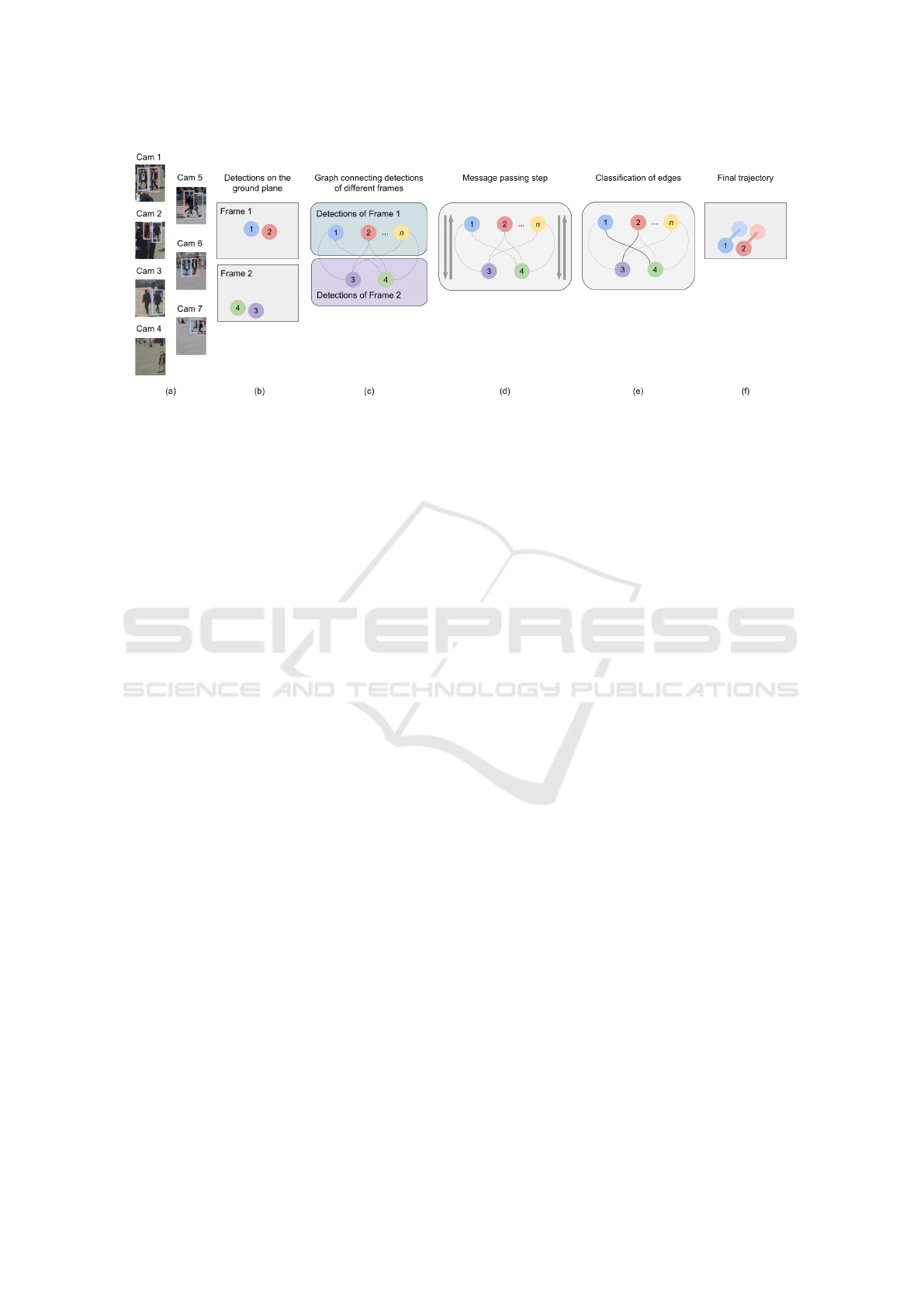
Figure 1: Overview of our approach. (a) Given a set of images from multiple cameras, we detect the 2D bounding boxes of

pedestrians in each camera and (b) project them onto the 3D world ground plane as proposed by Lima et al. (2021). Our task

is to identify which detections of different frames belong to the same pedestrian, therefore, (c) we create a graph where the

nodes represent the detections on the world ground plane, and the edges connect nodes from different frames. It is unnecessary

to have the same number of detections in each frame, e.g., Frame 1 can have n detections, and Frame 2 can have m detections.

Then, (d) we use the neural network architecture proposed by Bras

o & Leal-Taix

e (2020) to propagate the characteristics of

nodes and edges across the graph. (e) We use a sigmoid function to classify whether an edge is active or inactive, where an

active edge means that the detections belong to the same person. Finally, we assign the same id for detections connected by

an active edge. (f) Using the position of the previous frame and the current frame, we can observe the trajectory of pedestrians

on the 3D world ground plane.

is at most 4, with two hidden layers with 18 neu-

rons and an output layer with 16 neurons. Mean-

while, the other encoder MLP is used for nodes, and

we can use three different arrangements as input. One

option is to use visual features only, extracted using

ResNet50 (He et al., 2016) pre-trained in the Ima-

geNet dataset (Deng et al., 2009), where the size is

2048. Another one is to use pedestrian coordinates,

where the size is 2, and we also try to concatenate vi-

sual features with coordinates, where the size is 2050.

So then, the MLP has a hidden layer with 128 neurons

and an output layer with 32 neurons.

The update MLPs are responsible for learning the

function that better combines the characteristics of

nodes and edges. One update MLP is used for edges,

and it has an input layer with 96 neurons, a hidden

layer with 80 neurons, and an output layer with 16

neurons. Two update MLPs learn the attributes of past

and future nodes separately. They have an input layer

with 48 neurons, a hidden layer with 56 neurons, and

an output layer with 32 neurons. After obtaining the

updated attributes of the past and future nodes, an-

other update MLP concatenates both information and

transforms its size with an input layer of 64 neurons

and one output layer of 32 neurons.

The classiﬁer MLP produces a numeric output

used for classiﬁcation. It has an input layer with 16

neurons, a hidden layer with 8 neurons, and an output

layer with 1 neuron.

Figure 2 illustrates the architecture used. As men-

tioned earlier, the feature embeddings we use as node

attributes are extracted with ResNet50. We also ex-

perimented using pedestrian coordinates instead of

feature embeddings and concatenating features and

coordinates. Furthermore, we use the distance be-

tween frames, the geometric distance, and the appear-

ance distance for edges. The distance between frames

) is

= f

(B)

− f

(A)

, (1)

in which f

(A)

and f

(B)

are the frames where detections

A and B appeared. The geometric distance (d

) is the

distance between x coordinates and between y coordi-

nates

= x

(B)

− x

(A)

(2)

= y

(B)

− y

(A)

, (3)

where x

(A)

and x

(B)

are the x coordinates of detections

A and B, and d

is the x distance of their edge. The

same applies to d

, and together d

and d

are the ge-

ometric distance. The appearance distance (d

) is the

cosine distance between the visual features. These at-

tributes are the input to the encoder MLP.

As the nodes need to use one bounding box, and

in this work, we have several, they are stacked ver-

tically to turn into one input to ResNet50. However,

this neural network needs a ﬁxed-size input, but the

pedestrian can appear in different numbers of cam-

eras. So the input size is ﬁxed at the maximum size

considering the total number of cameras, and a vector

VISAPP 2023 - 18th International Conference on Computer Vision Theory and Applications

976

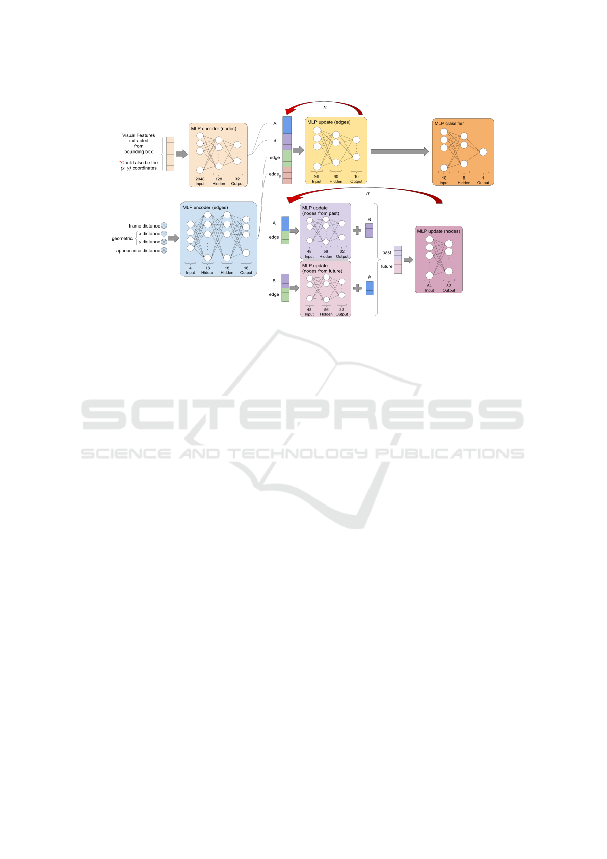
Figure 2: MPNN architecture. First, we extract visual features from detections and feed them to an encoder MLP. Instead of

this, we could have also used (x, y) coordinates. Similarly, we obtain edge characteristics by calculating the distance between

frames, between x, between y coordinates, and between visual features of the detections. They also feed another encoder MLP.

With the results of these encoders, we start the message-passing process, where we update node and edge characteristics n

times. At each message passing step, we concatenate features of node A, node B, the edge between A and B, and the initial

state of this edge (before any update). We use this as input to the MLP that will update the edge. With nodes, the update

starts separately for nodes from the past and future. Considering A is a detection from the past and B is from the future, we

concatenate A with its edge and pass it through the MLP that updates nodes from the past. Then, we use B and its edge to

update the MLP of nodes from the future. We sum each result with the node that was not used, concatenate them, and pass it

through an MLP that updates nodes. After the n steps, the ﬁnal edge is classiﬁed using a classiﬁer MLP.

of zeros replaces images from cameras without pedes-

trian detection. Also, each bounding box is resized to

128x64 before being stacked.

Then, for each pair of nodes A and B connected

by an edge, their attributes and the edge attributes are

concatenated and used as input to update the edges’

MLP. Initially, these attributes are the output of the

encoder MLP, but this MLP updates the edge at-

tributes, thus propagating the information from the

nodes to the edges.

Similarly, each pair of nodes A and B connected

by an edge updates the attributes of the nodes. How-

ever, this update considers the past and future rela-

tionship between them. First, we concatenate the at-

tributes of the nodes from the past with the edge at-

tributes. They are the input to the update MLP of

the nodes from the past. Its output sums with the at-

tributes of the nodes from the future. Afterward, the

attributes of the future nodes are concatenated with

the edge attributes and used as input for the update

MLP of the future nodes. Its output sums with the

attributes of the nodes from the past. This way, the

network is trained by differentiating past and future

information from pedestrians. Past and future results

are concatenated and used as input for the last update

MLP, which updates the node attributes.

This update phase can be repeated several times

and is the part that represents the MPNN process of

passing messages. The information obtained by nodes

and edges is shared and mixed.

Subsequently, the edge attributes are the input to

the classiﬁer MLP, and its output is used as the pa-

rameter of the sigmoid function to perform the binary

classiﬁcation of the edge between 0 (inactive) or 1

(active), which will determine whether the detections

connected by this edge are really from the same per-

son or not.

3.3 Training and Validation

We use the binary-cross-entropy loss function to cal-

culate how much the wrong predictions should be pe-

nalized. For each passage l, we calculate the penalty

for prediction ˆy

made for edge e, and then the penal-

ties for all edges are added together:

loss

(l)

= −

∑

e∈E

w·y

·log(ˆy

(l)

)+(1−y

)·log(1− ˆy

(l)

(4)

where E is the edge set and w is a weight that helps to

balance the loss when the number of active and inac-

tive labels is very different. This weight is calculated

Multi-Camera 3D Pedestrian Tracking Using Graph Neural Networks

977

by dividing the number of inactive labels by the num-

ber of active labels, which means that when there are

more inactive labels, the penalty for a wrong predic-

tion for an active label is more signiﬁcant. Also, the

negative logarithmic function has larger values when

it is close to zero, so when the label y

is 1, the loss

uses -log( ˆy

(l)

) because if ˆy

(l)

is zero the penalty will

be greater. If the label is 0, the loss is calculated with

-log(1 − ˆy

(l)

Then the penalty for all passages l will be added

together. Since this value is the loss of all edges, it is

divided by the number of edges to get the average loss

between a prediction ˆy

and a label y

loss( ˆy, y) =

|E|

∑

l=l

loss

(l)

. (5)

Training and validation were performed in two

ways. First, to compare the results obtained with dif-

ferent conﬁgurations, the network was trained using

70% of the frames present in the dataset as training,

20% as validation, and 10% as the test set.

Then, we use a 10-fold-cross-validation evalua-

tion with the conﬁguration that obtained the most ac-

curate result during the previous experiment. The 10-

fold-cross-validation consists of dividing the database

into ten datasets of equal size, running the training ten

times, and each run uses a different set as validation

and the others as training.

Furthermore, we trained the network running 25

epochs for each experiment with the Adam optimizer,

and the learning rate has been kept as l

= 10

−3

4 RESULTS

In this section, we describe the database and metrics

used in Subsection 4.1, report the experiments with

the pedestrian detector in Subsection 4.2, and the ex-

periments with the ground truth annotations in Sub-

section 4.3. We also compare our solution with re-

lated works in Subsection 4.4.

4.1 Dataset and Metrics

During experiments, we used the WILDTRACK

dataset (Chavdarova et al., 2018), which has seven

cameras with overlapping views in an open area with

an intense ﬂow of people. It has ground truth an-

notations that contain each pedestrian’s identiﬁcation

number, the coordinate pair (x, y) that represents its

3D position on the world ground plane, and its bound-

ing box on each camera through 400 frames.

The main metric used is multiple object tracking

accuracy (MOTA), which summarizes the relation-

ship between errors and total detections as follows:

MOTA = 1 −

FP + FN + MM

OBJ

, (6)

where FP is the number of false positives, FN is the

number of false negatives, MM is the number of mis-

matches, and OBJ is the number of objects in the

ground truth annotations.

Another metric used is multiple object tracking

precision (MOTP), which calculates tracking preci-

sion as

MOT P = 1 −

err

matches

, (7)

where d

err

is the sum of the geometric differences be-

tween the tracked position and the actual location, and

matches

is the number of cases where a match be-

tween the tracking and the ground truth annotation

occurred. Both metrics were proposed by (Bernardin

and Stiefelhagen, 2008). We observed them more dur-

ing experiments, but we also report the other MOT

Challenge benchmark metrics for completeness (Mi-

lan et al., 2016).

The experiments were carried out using a machine

that has an Intel Xeon processor @ 2.20GHz, 26GB

of RAM, and an NVIDIA Tesla P100 GPU with 16GB

of memory.

4.2 Experiments Using a Pedestrian

Detector

Using the detections obtained through a detection al-

gorithm, the solution proposed in this work can be

evaluated in the same way it would be used in prac-

tice. Therefore, ﬁrst, we used as the test set the de-

tections of (Lima et al., 2021). We train the neural

network with two variations, one using the ground

truth annotations and another using labels obtained

with the solution proposed by Lyra et al. (2022). The

latter is a tracking algorithm that results in detections

with assigned identities and would exempt the need

for ground truth annotations since this solution works

without training (Lyra. et al., 2022).

Tables 1 and 2 show the results obtained by train-

ing with the ground truth annotations and with Lyra et

al. (2022) tracker, respectively. The “Name” column

describes the conﬁguration used, where the number

(2 or 15) refers to the number of frames considered

in the graph construction. When we use 15 frames,

the algorithm uses both previous and future frames,

while when using 2 frames, we analyze the algorithm

using only the current and previous frames. We also

evaluated the algorithm’s performance using different

VISAPP 2023 - 18th International Conference on Computer Vision Theory and Applications

978

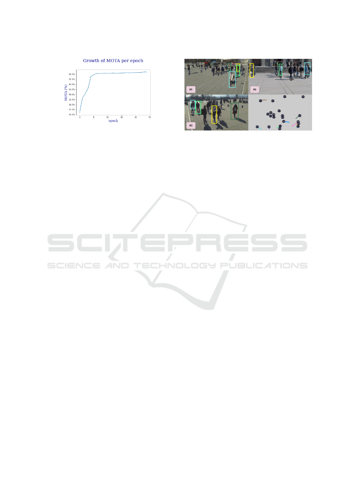
Figure 3: MOTA obtained at each iteration during 10-fold-

cross-validation.

parameters as edge characteristics. The distance be-

tween frames and the geometric distance are essential,

but we show the results of using and not using the ap-

pearance distance.

It is possible to observe that in both cases, the

best results were obtained when using 15 frames and

not using the appearance distance between detections.

When training with ground truth annotations, the pro-

posed solution reached 76.6% of MOTA, while when

training with Lyra et al. (2022) results, we achieved

77.1% of MOTA.

Also, training lasts approximately 3-6 minutes,

while inference processes around 40 fps. However, to

use the visual characteristics, it is necessary to process

the detections beforehand to obtain the Re-ID vectors,

and this makes the algorithm slower, reaching 0.6 fps.

Therefore, we also performed tests using only the x

and y coordinates as node attributes, and we obtained

similar results without changing the above framerate

of 40 fps. Besides, we try using coordinates and Re-

ID concatenated. For each conﬁguration, we execute

the test ten times, calculate the average MOTA and

the standard deviation (SD), and we apply the best

conﬁguration from Table 2 (15 + d

+ d

). The

results are on Table 3.

Considering the best conﬁguration, we exper-

imented with the 10-fold-cross-validation pattern,

where we averaged the results obtained in the ten parts

of training per iteration. The best MOTA achieved is

at epoch 24 with 62.3%. The evolution of MOTA is

illustrated in Figure 3.

Observing one frame of the inference obtained

after training with the previous best conﬁguration,

we analyzed the result qualitatively, highlighting four

pedestrians. Figure 4 shows cameras #1, #3, #5, and

the world ground plane corresponding to frame #364,

with pedestrians #009, #014, #019, and #024 colored

in yellow, light green, dark green, and light blue, re-

spectively. In these images, it is possible to see that in

addition to the pedestrians being re-identiﬁed in dif-

ferent cameras, they also continue to be tracked even

when they have severe occlusion. For example, in

Figure 4: Images from cameras #1, #3, #5, and the world

ground plane of frame #364 highlighting pedestrians #009,

#014, #019, and #024 in yellow, light green, dark green, and

light blue, respectively.

camera #5 (center image), pedestrian #024 is not seen

but has stable tracking in the world ground plane as it

continues appearing on other cameras.

Pedestrian #009 is next to pedestrians #006 and

#011, and pedestrian #006 is the one holding a bag in

camera #3. On camera #5, the person with the bag

is occluding pedestrian #009, but we notice that the

tracking of pedestrians #009 and #011 continues cor-

rectly.

Pedestrians #014 and #019 are more examples of

correct pedestrian tracking despite some cameras ex-

periencing partial or severe occlusions as they appear

in other cameras.

Also, despite the overall result being good, there

are still errors in tracking. For example, detection

#027 appears, but when we project it onto cameras

#1 and #3, we see that it points to an empty location,

so it is a false positive.

4.3 Experiments Using Ground Truth

Detection Annotations

As the quality of TBD trackers depends on the quality

of the detections, we also experimented with using the

neural network to track the ground truth annotations.

Table 4 displays the results, where the highest MOTA

is 99.9% with the same conﬁguration as the previous

experiments.

This result demonstrates how much the quality of

detections reﬂects on tracking, reaching a result that

is 22.9% better than the best result of previous exper-

iments and almost perfect.

4.4 Comparison with Related Works

In Table 5, we compare our results with state-of-the-

art methods in 10% of the WILDTRACK dataset.

The best results obtained are similar to the ones

Multi-Camera 3D Pedestrian Tracking Using Graph Neural Networks

979

Table 1: Results obtained in the test set after training with ground truth annotations.

Name MOTA MOTP IDF1 IDP IDR Rcll Prcn GT MT PT ML FP FN IDs FM

2+d

75.2% 90.7% 74.9% 73.9% 75.9% 90.8% 88.3% 41 29 10 2 114 88 32 23

2+d

73.7% 82.6% 67.9% 67.0% 68.8% 90.3% 87.9% 41 30 9 2 118 92 40 26

15+d

76.7% 90.9% 82.1% 81.0% 83.2% 90.8% 88.3% 41 28 11 2 114 88 20 24

15+d

75.9% 86.6% 79.6% 78.5% 80.7% 90.8% 88.3% 41 30 9 2 114 88 27 21

Table 2: Results obtained in the test set after training with the output of Lyra et al. (2022) tracking.

Name MOTA MOTP IDF1 IDP IDR Rcll Prcn GT MT PT ML FP FN IDs FM

2+d

75.8% 90.6% 76.8% 75.8% 77.8% 90.8% 88.3% 41 30 9 2 114 88 28 23

2+d

75.7% 90.5% 78.2% 77.2% 79.3% 90.8% 88.3% 41 30 9 2 114 88 29 23

15+d

77.1% 90.7% 82.4% 81.3% 83.5% 90.8% 88.3% 41 28 11 2 114 88 16 22

15+d

76.8% 90.6% 82.1% 81.0% 83.2% 90.8% 88.3% 41 30 9 2 114 88 19 23

Table 3: Results obtained changing nodes features.

Name MOTA ±SD

Coordinates 77.02% ±0.147

Re-ID 77.03% ±0.125

Coordinates + Re-ID 77.04% ±0.171

Table 4: Results obtained testing with ground truth annota-

tions.

Frames

Distance

MOTA MOTP

2 Yes Yes No 98.6% 99.9%

2 Yes Yes Yes 98.9% 99.9%

15 Yes Yes No 99.9% 100%

15 Yes Yes Yes 99.7% 100%

Table 5: Comparison of our solution with related works.

You & Jiang (2020) tracking speed includes the detection

stage, while Lyra et al. (2022) and Ours do not include it.

Technique

Tracking

Speed

MOTA MOTP

Chavdarova

et al. (2018)

Ofﬂine 72.2% 60.3%

You & Jiang

(2020)

15 FPS

w/ det

74.6% 78.9%

Vo et al.

(2021)

Ofﬂine 75.8% -

Lyra et al.

(2022)

20 FPS

w/o det

77.1% 96.4%

Ours

40 FPS

w/o det

77.1% 90.7%

Table 6: Comparison of our solution with Lyra et al. (2022).

Technique Detections MOTA MOTP

Lyra et al.

(2022)

Detector 77.1% 96.4%

Ours Detector 77.1% 90.7%

Lyra et al.

(2022)

Ground

Truth

Annotations

98.9% 98.7%

Ours Ground

Truth

Annotations

99.9% 100%

from (Lyra. et al., 2022). Their solution uses a de-

terministic algorithm with a ﬁxed result of 77.1% of

MOTA, while our solution obtained results that oscil-

late between 76.9% and 77.1%. However, our solu-

tion can track at a rate of 40 fps, while Lyra et al.

(2022) tracks pedestrians at 20 fps. Although we sug-

gest using the algorithm of Lyra et al. (2022) in our

solution, it is only required for training, not affecting

our inference time. Both frame rates do not include

the duration of the detection process. (You and Jiang,

2020) work tracks at 15 fps, where this frame rate in-

cludes the detection process, and the other solutions

are ofﬂine. Compared to Lyra et al. (2022), we also

obtained more accurate and precise results when test-

ing with ground truth detection annotations, as seen

in Table 6.

As the WILDTRACK dataset also has annotations

regarding the bounding boxes of each camera, we car-

ried out an experiment using the original algorithm by

Bras

o & Leal-Taix

e (2020) to track only the 2D de-

tections obtained by YOLOv3 in the ﬁrst camera of

WILDTRACK. The MOTA was 45.5%, demonstrat-

VISAPP 2023 - 18th International Conference on Computer Vision Theory and Applications

980

ing that the use of multiple cameras proposed in this

work signiﬁcantly improved this type of environment.

5 CONCLUSIONS

We proposed a new approach for 3D pedestrian track-

ing in multi-camera environments in this work. Our

method uses the MPNN architecture to associate de-

tections that belong to the same pedestrian and to

trace their spatial-temporal trajectory. By carrying

out experiments on the WILDTRACK database, we

showed that the technique reaches up to 77.1% of

MOTA when trained with the tracking result of Lyra

et al. (2022) and 62.3% of MOTA in 10-fold-cross-

validation. In addition, the time required to track

pedestrians is 40 fps, which is twice the most accu-

rate competing solution (Lyra et al. (2022)).

The results obtained considering only 2 frames are

worse than those obtained with 15 frames because

there are more identity changes, so it would be in-

teresting to study how to reduce these changes so that

the performance using 2 frames is as good as the one

when using 15 frames.

Furthermore, this work evaluated the use of a pos-

sible approach to training the neural network without

the need for ground truth annotations. However, sev-

eral unsupervised training techniques could be tried

in this scenario.

REFERENCES

Badue, C., Guidolini, R., Carneiro, R. V., Azevedo, P., Car-

doso, V. B., Forechi, A., Jesus, L., Berriel, R., Paix

ao,

T. M., Mutz, F., de Paula Veronese, L., Oliveira-

Santos, T., and De Souza, A. F. (2021). Self-driving

cars: A survey. Expert Systems with Applications,

165:113816.

Bergmann, P., Meinhardt, T., and Leal-Taixe, L. (2019).

Tracking without bells and whistles. In Proceedings of

the IEEE/CVF International Conference on Computer

Vision (ICCV).

Bernardin, K. and Stiefelhagen, R. (2008). Evaluating mul-

tiple object tracking performance: the clear mot met-

rics. EURASIP Journal on Image and Video Process-

ing, 2008:1–10.

Bras

o, G. and Leal-Taix

e, L. (2020). Learning a neural

solver for multiple object tracking. In Proceedings

of the IEEE/CVF Conference on Computer Vision and

Pattern Recognition (CVPR), pages 6247–6257.

Chavdarova, T., Baqu

e, P., Bouquet, S., Maksai, A., Jose,

C., Bagautdinov, T., Lettry, L., Fua, P., Van Gool, L.,

and Fleuret, F. (2018). Wildtrack: A multi-camera

hd dataset for dense unscripted pedestrian detection.

In Proceedings of the IEEE Conference on Computer

Vision and Pattern Recognition (CVPR), pages 5030–

5039.

Deng, J., Dong, W., Socher, R., Li, L.-J., Li, K., and Fei-Fei,

L. (2009). Imagenet: A large-scale hierarchical image

database. In 2009 IEEE conference on computer vi-

sion and pattern recognition (CVPR), pages 248–255.

IEEE.

Gan, Y., Han, R., Yin, L., Feng, W., and Wang, S. (2021).

Self-supervised multi-view multi-human association

and tracking. In Proceedings of the 29th ACM Inter-

national Conference on Multimedia, MM ’21, page

282–290, New York, NY, USA. Association for Com-

puting Machinery.

He, K., Zhang, X., Ren, S., and Sun, J. (2016). Deep resid-

ual learning for image recognition. In Proceedings of

the IEEE conference on computer vision and pattern

recognition (CVPR), pages 770–778.

Li, J., Wang, C., Zhu, H., Mao, Y., Fang, H.-S., and Lu,

C. (2019). Crowdpose: Efﬁcient crowded scenes pose

estimation and a new benchmark. In Proceedings of

the IEEE/CVF Conference on Computer Vision and

Pattern Recognition (CVPR), pages 10863–10872.

Lima, J. P., Roberto, R., Figueiredo, L., Simoes, F., and

Teichrieb, V. (2021). Generalizable multi-camera 3d

pedestrian detection. In Proceedings of the IEEE/CVF

Conference on Computer Vision and Pattern Recogni-

tion (CVPR), pages 1232–1240.

Lyra., V., de Andrade., I., Lima., J., Roberto., R.,

Figueiredo., L., Teixeira., J., Thomas., D., Uchiyama.,

H., and Teichrieb., V. (2022). Generalizable online

3d pedestrian tracking with multiple cameras. In Pro-

ceedings of the 17th International Joint Conference

on Computer Vision, Imaging and Computer Graphics

Theory and Applications - Volume 5: VISAPP,, pages

820–827. INSTICC, SciTePress.

Milan, A., Leal-Taix

e, L., Reid, I., Roth, S., and Schindler,

K. (2016). Mot16: A benchmark for multi-object

tracking. arXiv preprint arXiv:1603.00831.

Redmon, J. and Farhadi, A. (2018). Yolov3: An incremental

improvement. arXiv.

Sun, Z., Chen, J., Chao, L., Ruan, W., and Mukherjee, M.

(2020). A survey of multiple pedestrian tracking based

on tracking-by-detection framework. IEEE Transac-

tions on Circuits and Systems for Video Technology,

31(5):1819–1833.

Vo, M., Yumer, E., Sunkavalli, K., Hadap, S., Sheikh, Y.,

and Narasimhan, S. G. (2021). Self-supervised multi-

view person association and its applications. IEEE

Transactions on Pattern Analysis and Machine Intel-

ligence, 43(8):2794–2808.

You, Q. and Jiang, H. (2020). Real-time 3d deep multi-

camera tracking. arXiv preprint arXiv:2003.11753.

Zhang, X., Yu, Q., and Yu, H. (2018). Physics inspired

methods for crowd video surveillance and analysis: a

survey. IEEE Access, 6:66816–66830.

Zhou, X., Koltun, V., and Kr

ahenb

uhl, P. (2020). Tracking

objects as points. In Vedaldi, A., Bischof, H., Brox, T.,

and Frahm, J.-M., editors, Computer Vision – ECCV

2020, pages 474–490, Cham. Springer International

Publishing.

Multi-Camera 3D Pedestrian Tracking Using Graph Neural Networks

981