Quantum Reinforcement Learning for Solving a Stochastic Frozen Lake

Environment and the Impact of Quantum Architecture Choices

Theodora-Augustina Dr

agan

, Maureen Monnet

, Christian B. Mendl

2,3

and Jeanette M. Lorenz

Fraunhofer Institute for Cognitive Systems IKS, Munich, Germany

Technical University of Munich, Department of Informatics, Boltzmannstraße 3, 85748 Garching, Germany

Technical University of Munich, Institute for Advanced Study, Lichtenbergstraße 2a, 85748 Garching, Germany

jeanette.miriam.lorenz@iks.fraunhofer.de

Keywords:

Quantum Reinforcement Learning, Proximal Policy Optimization, Parametrizable Quantum Circuits, Frozen

Lake, Expressibility, Entanglement Capability, Effective Dimension.

Abstract:

Quantum reinforcement learning (QRL) models augment classical reinforcement learning schemes with

quantum-enhanced kernels. Different proposals on how to construct such models empirically show a promis-

ing performance. In particular, these models might offer a reduced parameter count and shorter times to reach

a solution than classical models. It is however presently unclear how these quantum-enhanced kernels as

subroutines within a reinforcement learning pipeline need to be constructed to indeed result in an improved

performance in comparison to classical models. In this work we exactly address this question. First, we pro-

pose a hybrid quantum-classical reinforcement learning model that solves a slippery stochastic frozen lake, an

environment considerably more difﬁcult than the deterministic frozen lake. Secondly, different quantum ar-

chitectures are studied as options for this hybrid quantum-classical reinforcement learning model, all of them

well-motivated by the literature. They all show very promising performances with respect to similar classical

variants. We further characterize these choices by metrics that are relevant to benchmark the power of quan-

tum circuits, such as the entanglement capability, the expressibility, and the information density of the circuits.

However, we ﬁnd that these typical metrics do not directly predict the performance of a QRL model.

1 INTRODUCTION

Reinforcement learning (RL) is one of the pillars of

machine learning, together with supervised and un-

supervised learning. It has many industry-relevant

applications, such as robotic tasks on assembly lines

(Christiano et al., 2016), drug design (Popova et al.,

2018), and navigation tasks (Zhu et al., 2017). When

applying RL to complex settings and environments,

there is currently a tendency to focus on approximate

solutions due to the complexity involved. In this con-

text, the use of (deep) neural networks (NN) as value

function approximators inside the policy of the RL

agent has gained in popularity. Here, the state of

the environment is processed by a NN in order to at-

tribute a value function to it, or to estimate the value

of each possible action to be taken from that state.

This leads to policy gradient algorithms such as Deep

Q-Networks (DQN) (Mnih et al., 2013) and Proximal

Policy Optimization (PPO) (Schulman et al., 2017),

which can even play video games such as “Space In-

vaders” (Mnih et al., 2013). The issues with these

approaches, however, is that they use increasingly

deep NNs, which may take several days of training

on a GPU for one problem instance (Ceron and Cas-

tro, 2021). With increasingly complex environments,

these methods may therefore experience scaling is-

sues. Hence, it is interesting to explore alternative

methods and directions.

The use of quantum computing (QC) subroutines

could be a promising path for RL. QC has theo-

retically been shown to exponentially or polynomi-

nally accelerate important subroutines, in particular

for search problems via Grover’s algorithm (Grover,

1996) or for solving systems of linear equations with

the HHL algorithm (Harrow et al., 2009). Moreover,

theoretical work (Caro et al., 2022) shows that certain

quantum algorithms and quantum-enhanced models

may lead to a better generalization than classical al-

gorithms in the case of a small training dataset. Fur-

ther work hints that quantum algorithms may be able

to observe new non-trivial characteristics in the data

agan, T., Monnet, M., Mendl, C. and Lorenz, J.

Quantum Reinforcement Learning for Solving a Stochastic Frozen Lake Environment and the Impact of Quantum Architecture Choices.

DOI: 10.5220/0011673400003393

In Proceedings of the 15th International Conference on Agents and Artiﬁcial Intelligence (ICAART 2023) - Volume 2, pages 199-210

ISBN: 978-989-758-623-1; ISSN: 2184-433X

 2023 by SCITEPRESS – Science and Technology Publications, Lda. Under CC license (CC BY-NC-ND 4.0)

199

(Liu et al., 2021), as well as to reach similar or better

results, while requiring less training steps (Heimann

et al., 2022).

Different successful proposals have been made on

how quantum algorithms could be integrated in RL

models. These can be distinguished into two main

directions, either trying to employ quantum search al-

gorithms as replacement for the agent (Niraula et al.,

2021), or replacing the NN part with a quantum cir-

cuit (Heimann et al., 2022). Possible application

ﬁelds include robot navigation tasks (Heimann et al.,

2022) or medical tasks. E.g., within the oncological

area, a proposal was made to adapt the radiotherapy

treatment plans of lung cancer patients depending on

how they have responded to previous treatments (Ni-

raula et al., 2021). However, none of the existing

works in quantum reinforcement learning (QRL) have

investigated the correlation between the performance

of the solution and the architecture of the quantum cir-

cuit yet. It is indeed unclear from the literature what

more or less promising architectures for quantum ker-

nels within a RL model might be.

Within this work, we investigate multiple addi-

tions to the ﬁeld. First, we deﬁne a variant of the

slippery frozen lake (FL) example (Brockman et al.,

2016), which is a signiﬁcantly more difﬁcult stochas-

tic environment in comparison to the typically used

deterministic FL. We then consider a variety of dif-

ferent hybrid quantum-classical (HQC) PPO mod-

els, where the NNs of the classical algorithm are re-

placed by parametrised quantum circuits (PQC). We

obtain good performance in comparison to the classi-

cal models considered, with respect to the number of

time steps required until training convergence and the

maximal reward reached during training. The quan-

tum circuits within these models are chosen following

suggestions from the literature about promising quan-

tum circuits (Sim et al., 2019), which e.g., are more

efﬁcient in using present-term quantum hardware, or

may solve speciﬁc subproblems. We then characterise

the solution with quantum-related metrics such as en-

tanglement capability, expressibility, and effective di-

mension. We ﬁnd that although all quantum circuits

show a promising performance, the gain in perfor-

mance does not seem to directly correlate to these

quantum metrics. Therefore, our work can only give

a ﬁrst indication for promising quantum architectures

in QRL.

This paper is structured as follows: the next sec-

tion will present the related work and current status of

using quantum computing in RL. The third section in-

troduces the slippery FL environment and the pipeline

of our PPO-based solution. Section four details the

results achieved by our HQC PPO model. The ﬁfth

section ﬁrst deﬁnes the three quantum metrics used,

and then looks at the correlation with the results ob-

tained. Finally in the sixth section we present conclu-

sions and propose possible future research directions.

2 RELATED WORK

In the stream of HQC RL solutions that use quantum

search algorithms, a model in the oncological area has

been presented by (Niraula et al., 2021). The goal is

to adapt the last two weeks of a radiotherapy treat-

ment plan depending on the patient’s reaction to the

ﬁrst four weeks of treatment. The need for artiﬁ-

cial intelligence methods comes from the fact that nu-

merous biological factors can inﬂuence the individual

impact of the treatment. The proposed solution uses

Grover’s search to decide the next step in the course

of the treatment by taking into account the current re-

sponse. Oncological metrics were evaluated in order

to maximise the treatment outcome and optimise its

efﬁciency. In this particular case, QC is not used to

accelerate the calculation, but to improve the preci-

sion.

A second direction in QRL considers replacing

NNs by quantum circuits. Such methods have shown

an interesting potential to solve complex tasks while

requiring less computational resources than classical

RL models (Jerbi et al., 2021; Chen et al., 2020;

Lockwood and Si, 2020). In these cases, quantum

circuits are used for approximating both policy and

value functions.

In (Chen et al., 2020), the authors suggest using

PQCs instead of NNs in the DQN algorithm (Mnih

et al., 2015). The expectation values of the PQC

are measured and associated to the Q function of the

DQN algorithm. They obtain promising results in

solving a shortest-path deterministic FL and a Cog-

nitive Radio (Gawłowicz and Zubow, 2019) environ-

ment.

Alternatively, (Jerbi et al., 2021) replace the pol-

icy of a classical RL algorithm (Sutton and Barto,

2018) with a PQC, while computing the value func-

tion classically. This work also employs the idea of a

data re-uploading circuit (P

erez-Salinas et al., 2020)

in the PQC, where data embedding and variational

parts are sequentially repeated to increase the over-

all complexity of the PQC. The authors benchmark

two different hybrid quantum architectures against the

maximal reward obtained during learning on Gym en-

vironments (Brockman et al., 2016). While this work

shows a promising hybrid advantage on two environ-

ments, it is not thoroughly tested against classical so-

lutions. Nevertheless, one can clearly observe how

ICAART 2023 - 15th International Conference on Agents and Artiﬁcial Intelligence

200

architectural choices and hyperparameters such as cir-

cuit depth can impact the performance.

A hybrid data re-uploading technique can also

help a robot agent to navigate through a maze-like en-

vironment and reach a desired solution, while avoid-

ing obstacles (Heimann et al., 2022). In this work,

both of the NN function approximators of the Double

Q-learning algorithm (Van Hasselt et al., 2016) were

replaced with a hybrid module containing a PQC fol-

lowed by a post-processing layer. The results of the

hybrid solution are competitive with the ones a clas-

sical solution, reaching the reward threshold after a

similar number of training steps. Moreover, the hy-

brid solution needs 10 times fewer trainable parame-

ters to solve the environment.

3 SOLVING A SLIPPERY

FROZEN LAKE

ENVIRONMENT

3.1 The Slippery Frozen Lake

The FL environment is a common benchmark ex-

ample in classical RL (Steckelmacher et al., 2019;

Khadke et al., 2019; Gupta et al., 2021). The task

consists of navigating through a maze e.g., of size

4x4 in this study. The maze contains four types of

discrete tiles, including the start (S), the goal (G), the

tiles with holes (H) to be avoided, and the frozen tiles

the agent can walk across (F). A previous example

of solving this environment by QRL reduced the task

to a deterministic environment, where the agent navi-

gating through the maze would always move into the

direction desired (Chen et al., 2020). We found that

even for present small QRL models, this is a fairly

simple task to solve. Therefore, we opted for a signiﬁ-

cantly more difﬁcult slippery FL environment (Brock-

man et al., 2016), which is stochastic in nature. In the

default stochastic FL, the probability to slip and con-

sequently to move to an orthogonal direction to the

one desired is

. To mimic real environments more

closely, we reduced the probability to slip in this study

to 20%, as shown in Fig. 2.

The tiles and thus the possible states of the envi-

ronment are integers from 0 to 15. From any position,

the agent can go left, down, right or up. If the agent

moves to a hole, it receives a ﬁnal reward of 0 and the

learning process terminates. If the agent reaches the

goal, it receives a reward of 1. Moving across the lake

on the S and F tiles results in a 0 reward.

In order to control the quality of the agent that

learnt to navigate through an environment, usually a

reward threshold is established. If the reward obtained

by the agent is equal to or surpasses a given thresh-

old, the agent is considered to have successfully learnt

the environment. The reward threshold is calculated

based on the average reward obtained when following

the optimal policy. Therefore, we ﬁrst determined the

optimal policy for our slippery FL environment and

averaged its rewards over 1000 test episodes. With

the resulting average reward of 0.85, we deducted a

reasonable reward threshold of 0.81, in a similar way

as done in the FL documentation (Brockman et al.,

2016).

3.2 The Architecture of the HQC

Solution

To solve our slippery FL environment, we designed a

hybrid PPO algorithm. The PPO algorithm was cho-

sen as a basis since it achieved the highest average re-

wards for many Gym environments (Schulman et al.,

2017), in comparison to other policy gradient meth-

ods. The PPO implementation used was provided by

the Stable Baselines 3 Python library (Rafﬁn et al.,

2021).

The ﬁrst experiments were performed without any

quantum kernel to create classical baselines. Here,

the policy and value function approximators are NNs

with two hidden layers of either 2, 4, 8, and 16 neu-

rons each, followed by a post-processing linear layer.

The relatively low number of neurons was chosen to

enable a fairer comparison with the hybrid variants

with quantum kernels, as these require a relatively

small number of trainable parameters. The input to

the classical solution is an one-hot vector encoding of

the state.

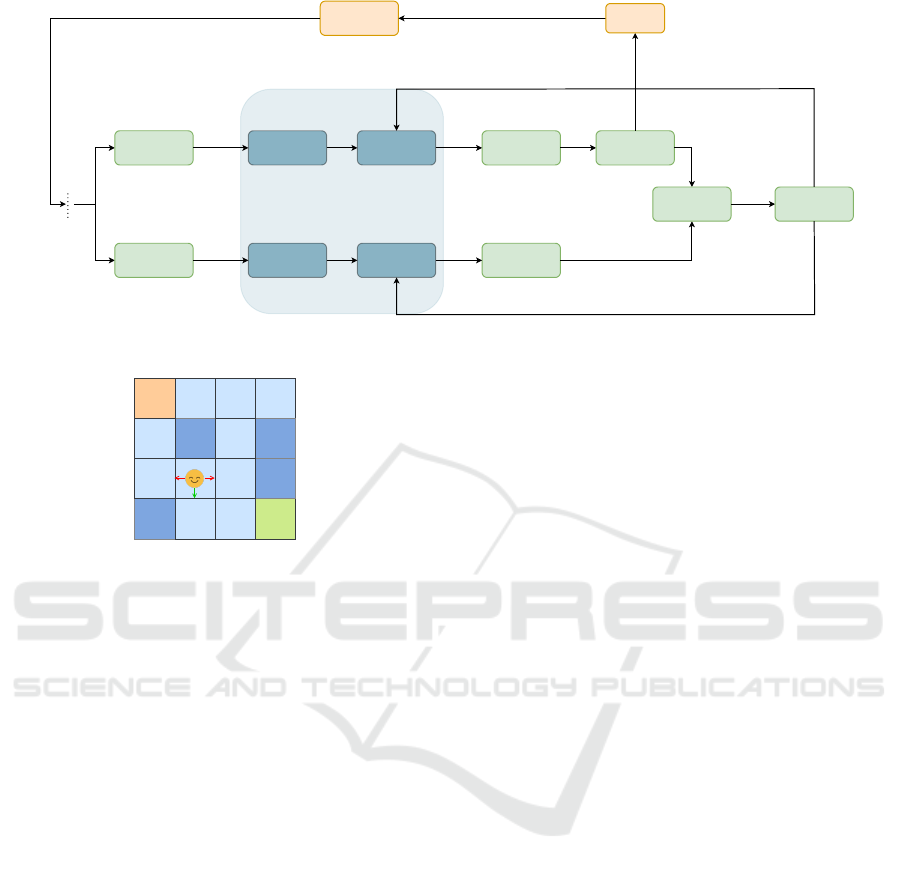
In the HQC solution, the algorithm remains the

same except for the policy and the value NNs, which

are replaced by quantum kernels, as shown in Fig. 1.

The quantum kernels consist of a data encoding, the

trainable PQC, a measurement step, and a classical

post-processing. The data encoding is done via basis

embedding using R

and R

gates. The state index

s is transformed into its binary representation s

bin

, and is used to turn the default

0000

⟩

input

state into the ψ

⟩

state. This is achieved

by setting the rotational parameters of the R

(θ) and

(θ) gates acting on wire i to θ = 0, if s

= 0, and

to θ = π if s

= 1. This ψ

state is the input to the

trainable parts of the circuits, which are the Policy

PQC and Value PQC of Fig. 1.

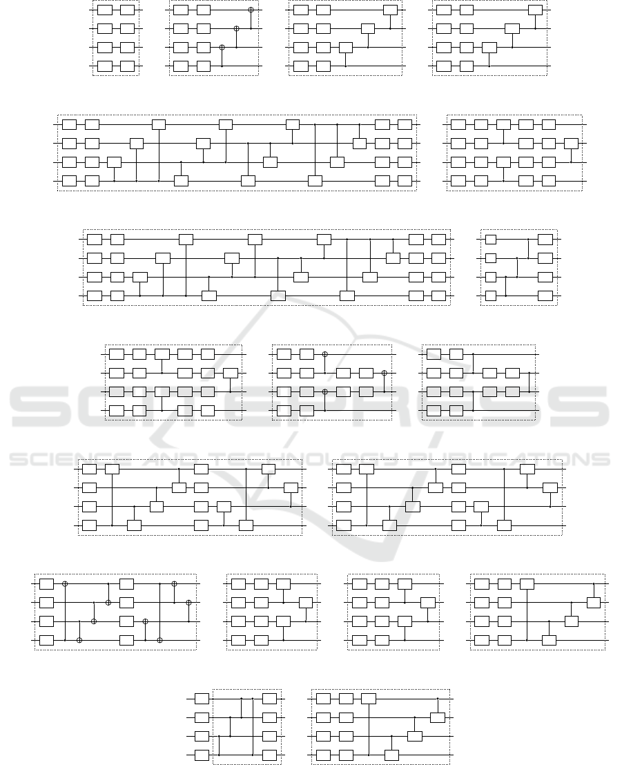
The circuit architectures are taken from the 19 cir-

cuits proposed in (Sim et al., 2019) and are shown in

Fig. 3. An argument put forward by the authors is

that these circuits were already designed for and suc-

Quantum Reinforcement Learning for Solving a Stochastic Frozen Lake Environment and the Impact of Quantum Architecture Choices

201

Binary

Conversion

Binary

Conversion

Basis

Embedding

Basis

Embedding

bin

Policy PQC

Value PQC

4 x 4

Linear Layer

4 x 1

Linear Layer

Quantum Module

Categorical

Distribution

π(s, a

)

Loss

Computation

Adam

Optimizer

V(s)

update trainable

parameters Θ

update trainable

parameters Θ

Environment

π(s, a

)

bin

Agent

a' = argmax

π(s, a)

Figure 1: The entire pipeline of our solution.

GH F

F F

1 2 3

F H

14 1512 13

8 9 11

80%

10% 10%

GH F

F F

1 2 3

F H

14 1512 13

8 9 11

80%

10% 10%

Figure 2: The structure of the FL for the state s = 9.

cessfully applied to diverse tasks. Moreover, all cir-

cuits are designed to be implementable on presently

or soon available Noisy Intermediate-Scale Quan-

tum (NISQ) devices, at various implementation costs.

Four different entanglement gates are used: CRX,

CRZ, CNOT, and CZ and ﬁve different entanglement

topologies: linear, all-to-all, pairwise, circular, and

shifted-circular-alternating. These categories are un-

derstood as they are deﬁned in the Qiskit documenta-

tion (Anis et al., 2021).

Circuit 1 is a basic quantum circuit with no en-

tanglement and two degrees of freedom, with rota-

tions around the X and Z axes of the Bloch sphere

for each qubit. Circuit 2, 3, and 4 were designed

by adding a basic linear entanglement using 3 differ-

ent entanglement gates, with the purpose of studying

the variation of the values of the quantum metrics for

each type of entanglement gate and with respect to

the ﬁrst circuit. Circuits 5 and 6 were introduced as

programmable universal quantum circuits in (Sousa

and Ramos, 2006) and used as quantum autoencoders

in (Romero et al., 2017). Circuits 7 and 8 are part

of the QVECTOR algorithm for quantum error cor-

rection (Johnson et al., 2017) and circuit 9 was intro-

duced as a ”Quantum Kitchen Sinks” quantum ma-

chine learning architecture to be used on NISQ de-

vices in (Wilson et al., 2018). The tenth circuit is

taken from a hardware-efﬁcient quantum architecture

introduced in (Kandala et al., 2017) as a variational

quantum eigensolver, used to ﬁnd the ground state en-

ergy for molecules. Circuits 11 and 12 are Josephson

samplers deﬁned in (Geller, 2018) , whose purpose is

to embed a vector of real elements into an n-qubits

entangled state. Finally, circuits 13, 14, 15, 18, and

19 were constructed based on the generic model cir-

cuit architecture for classiﬁcation tasks described in

(Schuld et al., 2020). Circuit 16 and 17 are derived

from circuits 3 and 4, but with the order of the last

two controlled entanglement gates swapped. The pur-

pose was to display the different expressibility values

of circuits 3 and 16 and circuits 4 and 17 and empha-

sise that not only the type, but also the position of the

quantum gates is important in a PQC.

After the trainable PQCs acted on ψ

, the expec-

tation value of the states are measured in the compu-

tational basis. The results are fed into a 4x4 linear

layer in the case of the policy function. This linear

layer outputs logits, which when normalised become

the probabilities to choose an action between (left,

down, right, up). This is thus the output of the pol-

icy function π. In the case of the state value function,

the layer post-processing the expectation values has a

4x1 dimension to output only one value for an input

state and to thus successfully model the value func-

tion approximator V . The loss is computed from the

π and V function values and then used to classically

adjust the parameters of the two PQCs accordingly.

This pipeline is shown in Fig. 1.

4 PERFORMANCE OF HQC

MODELS

For each classical and HQC architecture, three ex-

periments were executed. The reward was sampled

ICAART 2023 - 15th International Conference on Agents and Artiﬁcial Intelligence

202

⟩

Circuit 1

⟩

Circuit 2

⟩

Circuit 3

⟩

Circuit 4

⟩

Circuit 5

⟩

Circuit 7

⟩

Circuit 6

⟩

Circuit 9

⟩

Circuit 8

⟩

Circuit 11

⟩

Circuit 12

⟩

Circuit 13

⟩

Circuit 14

⟩

Circuit 15

⟩

Circuit 16

⟩

Circuit 17

⟩

Circuit 18

⟩

Circuit 10

⟩

Circuit 19

Figure 3: All 19 benchmarking quantum circuits, as presented in (Sim et al., 2019). These are the trainable part of the quantum

kernel in the HQC RL solution. The input of each of these circuits is the output state of the basis embedding that encodes the

state of the environment.

Quantum Reinforcement Learning for Solving a Stochastic Frozen Lake Environment and the Impact of Quantum Architecture Choices

203

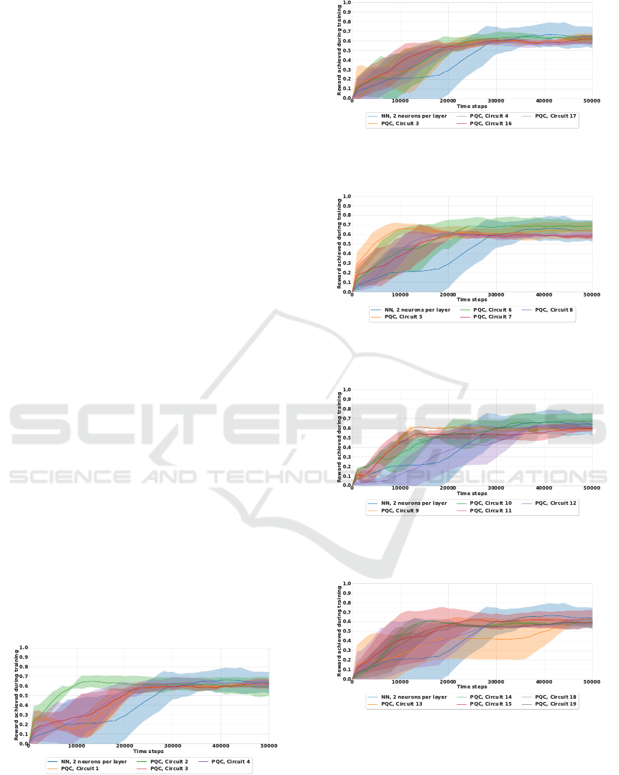
every 1000 time steps, and every experiment was

ran for a total of 50000 time steps. These results

were smoothed by a moving average over 10 data

points. The error bands are calculated using the stan-

dard error of the reward achieved at a particular time

step across all three experiments for a given architec-

ture. No hyperparameter tuning was performed in this

study due to the prohibitively long training times.

The RL metrics characterizing the performance of

each solution variant are the maximum reward (MR)

achieved during training and the time to convergence

(TTC). The time to convergence is deﬁned as the time

step when the reward stabilises around its highest

point. It is calculated as the ﬁrst time step where a re-

ward is reached that is not modiﬁed by more than 0.2

for all future time steps. The rewards for all quantum

circuits are plotted in Figs. 4 to 8 and detailed in Ta-

ble 1. In general, the HQC solutions and the classical

solutions achieved around the same average MR: the

best value was 0.86 for the classical approach using

four neurons per hidden layer and 0.85 for the HQC

algorithm when considering circuit 6 from Fig. 3.

Both types of solutions were successful and passed

the computed learning threshold of r

thr

= 0.81. Nev-

ertheless, when also considering the number of train-

able parameters, one can see that the HQC approach

only needs a third of the number of trainable param-

eters necessary for the classical one to perform com-

paratively well – 81 compared to 237 trainable param-

eters. Moreover, the TTC is clearly smaller for most

of the variants of HQC variants tested, as shown in

Figs. 4 – 8. The lowest mean TTC is 10330 time

steps for the HQC solution of circuit 2 with 41 train-

able parameters. In order to achieve stabilization that

fast, a classical solution would require 1245 trainable

parameters. Generally, the best HQC solutions were

the ones employing circuits 2, 6, and 10. Circuits 7-19

generally learn faster than the classical solution with a

much higher reward in the ﬁrst 25000 time steps, but

stabilise afterwards at a lower reward in our tests.

Figure 4: Comparison between the classical NN-based RL

solution and the HQC solutions using PQCs 1 to 4 respec-

tively, smoothed using a moving average.

Figure 5: Comparison between the classical NN-based RL

solution and the HQC solutions using PQCs 3, 4, 16, and

17, smoothed using a moving average.

Figure 6: Comparison between the classical NN-based RL

solution and the HQC solutions using PQCs 5 to 8 respec-

tively, smoothed using a moving average.

Figure 7: Comparison between the classical NN-based RL

solution and the HQC solutions using PQCs 9 to 12 respec-

tively, smoothed using a moving average.

Figure 8: Comparison between the classical NN-based RL

solution and the HQC solutions using PQCs 13 to 19 re-

spectively, smoothed using a moving average.

5 THE DEPENDENCE OF

PERFORMANCE ON

QUANTUM METRICS

The circuits proposed in (Sim et al., 2019) were de-

signed for different purposes and indeed show dis-

ICAART 2023 - 15th International Conference on Agents and Artiﬁcial Intelligence

204

Table 1: The results of all architectures used to solve the FL, evaluated with respect to the MR and the TTC (in thousands

of time steps) obtained during training. The MR and TTC values are obtained from the initial training processes, before the

smoothing that leads to Figs. 4 to 8. We also present the number of the trainable weights of each solution (W), together with

their expressibility (Exp), entanglement capability (Ent), and the effective dimension (ED). The results below are in ascending

order from the best to the worst values of the TTC and are grouped into classical and HQC solutions. For the quantum metrics,

the higher the Ent and ED values, and the lower the Exp values, the better the circuit is in reference to the respective metric.

The degree of correlation between the number of weights W and the MR and TTC of each solution remains for now unclear.

Solution W MR TTC Ent Exp ED

PQC–2 41 0.77 ± 0.16 10.33 ± 7.58 0.81 0.28 3.50

PQC–5 81 0.78 ± 0.22 11.33 ± 3.79 0.41 0.06 6.91

PQC–11 49 0.71 ± 0.20 12.33 ± 5.17 0.73 0.13 5.08

PQC–9 33 0.75 ± 0.02 12.50 ± 1.24 1.00 0.67 3.48

PQC–8 63 0.72 ± 0.08 14.33 ± 10.34 0.39 0.08 6.24

PQC–19 49 0.71 ± 0.07 14.33 ± 12.50 0.59 0.08 6.29

PQC–7 63 0.72 ± 0.06 15.33 ± 16.16 0.33 0.09 5.82

PQC–14 57 0.78 ± 0.25 16.33 ± 7.58 0.66 0.01 7.68

PQC–15 41 0.76 ± 0.28 19.67 ± 16.54 0.82 0.19 4.60

PQC–16 47 0.78 ± 0.09 20.00 ± 25.21 0.35 0.26 3.73

PQC–18 49 0.72 ± 0.10 20.00 ± 26.28 0.44 0.23 3.70

PQC–1 41 0.72 ± 0.10 21.67 ± 10.34 0.00 0.29 3.29

PQC–4 47 0.81 ± 0.18 23.67 ± 14.12 0.47 0.13 5.58

PQC–17 47 0.72 ± 0.09 25.00 ± 9.93 0.4 0.13 5.74

PQC–13 57 0.72 ± 0.08 25.00 ± 53.79 0.61 0.05 7.07

PQC–6 81 0.85 ± 0.16 26.00 ± 4.96 0.78 0.00 7.79

PQC–12 49 0.75 ± 0.19 26.66 ± 27.92 0.65 0.20 4.91

PQC–3 47 0.79 ± 0.06 27.67 ± 48.25 0.34 0.24 3.72

PQC–10 41 0.81 ± 0.27 31.67 ± 14.34 0.54 0.22 3.98

NN–16 1245 0.81 ± 0.10 11.33 ± 3.12 – – 48.78

NN–2 125 0.84 ± 0.04 19.00 ± 15.51 – – 42.53

NN–4 237 0.86 ± 0.00 22.00 ± 5.61 – – 72.13

NN–8 509 0.85 ± 0.02 24.33 ± 6.84 – – 74.83

tinct performances in our tests. Different metrics are

discussed in the literature to describe the power of

speciﬁc quantum circuits – comparing to other quan-

tum circuits, but in part also allow the comparison

to alternative classical implementations. It is how-

ever unclear from the literature if these metrics are

correlated with the performance of a QRL model or

not. Therefore, currently indications how a quantum

kernel should be constructed inside a QRL model are

missing. There are in particular three metrics that are

commonly discussed to characterise the properties of

quantum circuits:

1. Expressibility: This metric measures how well a

PQC covers the entire Hilbert space and therefore

indicates if the model would theoretically be able

to learn a target function.

2. Entanglement capability: The power of using

quantum circuits in comparison to classical vari-

ants also arises from the possibility to entangle

qubits, and to therefore strongly correlate them.

One may thus wonder if a higher entanglement

within a PQC leads to an improved performance

of the ﬁnal model.

3. Effective dimension: The effective dimension

allows a direct comparison of classical NN and

quantum neural networks (QNN) (i.e., PQC) by

interpreting both of them as statistical models

where one can measure the information capac-

ity. It is known (Abbas et al., 2021) that speciﬁc

QNNs exhibit a higher effective dimension than

equivalent classical models and that the concerned

QNNs may show a better performance .

In the following, we brieﬂy describe the mathe-

matical deﬁnitions of these metrics. Afterwards, we

discuss their correlation with the performance of our

QRL models.

5.1 Expressibility

The expressibility of a circuit (Sim et al., 2019) mea-

sures how well a set of (pure) states, here generated by

the PQC, covers the entire Hilbert space. The precise

calculation is described in (Sim et al., 2019). The cal-

culation uses the Kullback-Leibler (KL) divergence

Quantum Reinforcement Learning for Solving a Stochastic Frozen Lake Environment and the Impact of Quantum Architecture Choices

205

(Kullback and Leibler, 1951) between two distribu-

tions of ﬁdelities. These belong to the Haar ensemble

of random states and respectively to the ensemble of

states generated by the PQC. After having chosen a

PQC architecture, one uniformly samples two param-

eter vectors θ

and θ

from the entire parameter space

of the PQC. Then the ﬁdelity of their corresponding

states

⟩

and





is computed. This process is re-

peated multiple times and the results are afterwards

plotted as a histogram of the probability density func-

tion. For the Haar ensemble, the analytic probability

density function of ﬁdelities is

Haar

= (N − 1)(1 −F)

(N−2)

, (1)

where F is the ﬁdelity and N is the dimension of

the Hilbert space. Finally, the KL divergence is cal-

culated from the two histograms and the result is

the D

divergence, whose value is inversely propor-

tional to how expressive the circuit is:

Exp = D

PQC

(F;θ) || P

Haar

(F)). (2)

5.2 Entanglement Capability

In order to quantify the degree of entanglement, the

authors of (Sim et al., 2019) employed the Meyer-

Wallach (MW) entanglement measure (Meyer and

Wallach, 2002). The equation to assess the entangle-

ment capability is

Ent =

|S|

∑

∈S

⟩

), (3)

where S = {θ

} is the set of sampled parameter vec-

tors θ

, and Q is the MW measure. It is deﬁned as

⟩

)

∑

j=1

D(ι

(0)

⟩

, ι

(1)

⟩

), (4)

where n is the number of qubits in the system and D

is the generalised distance:

⟩

) =

∑

i, j

− u

. (5)

The linear mapping ι

(b) acts on a quantum basis

state:

(b)

. .. b

⟩

= δ



. .. b

j−1

j+1

. .. b



, (6)

where the b

qubit disappears and δ is the Kronecker-

Delta operator.

5.3 Effective Dimension

The Effective Dimension (ED) characterises both

classical and quantum machine learning models in

terms of their power to generalise and ﬁt to the given

data. It is derived from the Fisher Information Matrix

(FIM), which is a metric in statistics that assesses the

impact of the variance of the parameters of the model

on its output. In our case, it is computed using the

probability p(x, y; θ), which shows the relationship

between the input x ∈ R

, the output y ∈ R

out

, and

the parameters θ. The Riemannian space of the model

parameters is Θ ⊂ R

. The FIM is then computed as

F(θ) = E



∂

∂θ

log p(x, y; θ)

∂

∂θ

log p(x, y; θ)



(7)

where F ∈ R

d×d

. If one uses ﬁnite sampling, the FIM

can be approximated empirically to

(θ) =

∑

j=1

∂

∂θ

log p(x

, y

; θ)

∂

∂θ

log p(x

, y

; θ)

(8)

where k is the number of independent and identi-

cally distributed (i.i.d) samples (x

, y

) drawn from

p(x, y; θ). The formulation of the ED is based on

(Berezniuk et al., 2020). The authors of (Abbas et al.,

2021) extend this by adding the constant γ ∈ (0, 1] and

a log n term to assure the ED is bounded. This results

in the ﬁnal form we use in this work:

γ,n

) =

log(

det(id

γn

2πlogn

F(θ)) dθ)

log(

γn

2πlogn

)

(9)

where n > 1 ∈ N is the number of data samples, V

dθ is the volume of the parameter space, and

F(θ)

is the normalised FIM formulated as:

i j

(θ) = d

tr(F(θ)) dθ

i j

(θ). (10)

5.4 Impact of the Metrics on the

Performance

Values for the expressibility and the entanglement

capability for all considered circuits can be directly

taken from (Sim et al., 2019). The ED in contrast is

calculated by us. These three metrics are displayed in

Table 1 alongside the MR and TTC values, as well as

comparatively plotted in Figs. 9 to 14.

We ﬁrst observe that circuits 2, 3, and 4 largely

overcome circuit 1 – the circuit with no entanglement

– in MR, as expected. Similarly, circuit 2 performs

signiﬁcantly better than circuit 3 in the TTC (while

having a similar MR). The expressibility and ED of

the two circuits being comparable, this seems to in-

dicate that the entanglement capacity plays a positive

role in the ﬁnal performance. It is interesting to note

that circuits 2 and 4 are very similar in structure, while

ICAART 2023 - 15th International Conference on Agents and Artiﬁcial Intelligence

206

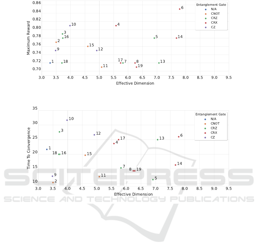
Figure 9: Correlation between the ED of a PQC and the MR obtained by the agent employing it, labeled using the PQC index

and aggregated by the entanglement gate.

Figure 10: Correlation between the ED of a PQC and the TTC obtained by the agent employing it, labeled using the PQC

index and aggregated by the entanglement gate.

circuit 4 containing three more trainable parameters

than circuit 2. The last three gates perform rotations

around the x-axis in case of both circuits. Despite this

similarity, circuit 4 with more trainable parameters re-

sults in a worse performance in the TTC than circuit

When inspecting the performance of further cir-

cuits, we do not observe a clear correlation between

the MR, the TTC, and the values of expressibility,

entanglement capacity, and effective dimension, as

shown in Figs. 9 to 14. For example, the best per-

forming circuit considering the average MR is circuit

6. It also has the best expressibility, the highest ED,

and the fourth highest entanglement capability, which

would seem to indicate a positive correlation. On the

other hand, circuit 13, one of the worse performing

circuits in MR, has a better expressibility, a higher en-

tanglement capability, and a higher effective dimen-

sion than circuit 10, which is, along with circuit 6,

one of the best performing circuits in MR.

In terms of the TTC, we ﬁnd circuits supporting

the hypothesis that better metrics lead to improved

performance, such as circuit 2 and its large entangle-

ment capacity; as well as counterexamples, such as

circuit 5, which is the second fastest in TTC, but is

overcome in all three metrics by circuit 6 (and with

exactly the same number of trainable parameters).

Additionally, in view of the dissimilar performances

between circuits 3 and 16 as well as circuits 4 and 17,

we deduce that the position of the entangling gates

can impact the performance, which is a factor that is

not considered in the three chosen metrics.

6 CONCLUSIONS

This work presents a hybrid quantum-classical rein-

forcement learning algorithm that successfully solves

a stochastic slippery 4x4 frozen lake example with a

probability of 80% to move into the desired direction

and 20% to move into undesired orthogonal direc-

tions. The algorithms considered achieve a maximum

Quantum Reinforcement Learning for Solving a Stochastic Frozen Lake Environment and the Impact of Quantum Architecture Choices

207

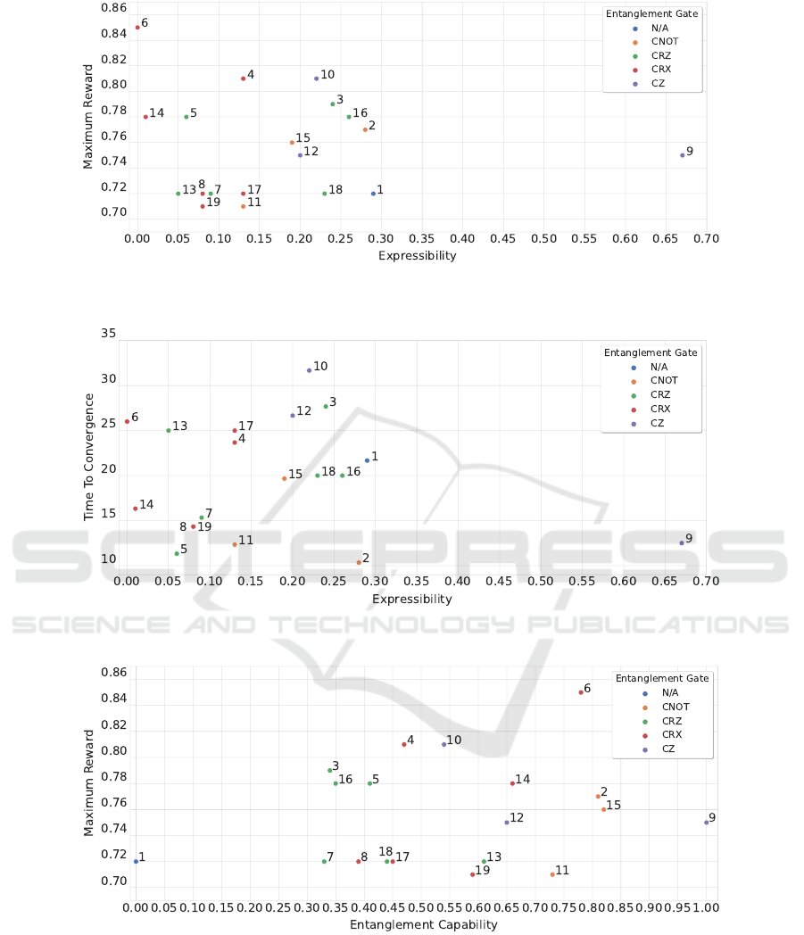
Figure 11: Correlation between the expressibility of a PQC and the MR obtained by the agent employing it, labeled using the

PQC index and aggregated by the entanglement gate.

Figure 12: Correlation between the expressibility of a PQC and the TTC obtained by the agent employing it, labeled using

the PQC index and aggregated by the entanglement gate.

Figure 13: Correlation between the entanglement capability of a PQC and the MR obtained by the agent employing it, labeled

using the PQC index and aggregated by the entanglement gate.

reward comparable to classical solutions while only

requiring a third of the number of trainable parame-

ters and also converging faster. In constructing the hy-

brid quantum-classical RL model, the internal policy

of the agent was replaced by a parametrised quantum

circuit. Different architectures were considered for

the parametrised quantum circuit. We found that three

of the hybrid quantum-classical variants solve the en-

vironment. We examined if this performance could

be explained by the quantum-speciﬁc metrics like ex-

pressibility, entanglement capability, or the effective

dimension. The latter is particularly interesting since

ICAART 2023 - 15th International Conference on Agents and Artiﬁcial Intelligence

208

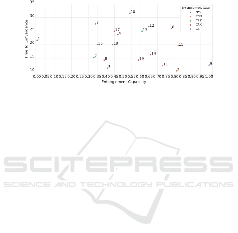
Figure 14: Correlation between the entanglement capability of a PQC and the TTC obtained by the agent employing it, labeled

using the PQC index and aggregated by the entanglement gate.

it allows the comparison of classical and quantum-

classical architectures. We ﬁnd however that the per-

formance is not directly linked to these metrics, which

could be because some additional factors inﬂuencing

the performance were missed by this study. There-

fore, presently the question on which parametrised

quantum circuit to use inside a RL model can only

be answered empirically.

Future work has to explore multiple directions.

First, this work only considered the simple basis en-

coding, but it will be interesting to investigate the

impact of different encoding techniques on the per-

formance metrics. Furthermore, the PPO algorithm

could be replaced by a simpler policy gradient one,

where the contribution of the quantum kernel to the

solution could possibly be better observed. Addition-

ally, so far, the work was done using only simula-

tions, without any attempts yet to run the algorithms

on quantum hardware. This was due to long wait-

ing times and a high number of iterations required be-

tween quantum hardware and classical systems. An

orthogonal research direction is to consider more so-

phisticated environments towards more realistic use

cases and situations and to therefore bring QRL tech-

niques closer to application.

ACKNOWLEDGEMENTS

The research is part of the Munich Quantum Valley,

which is supported by the Bavarian state government

with funds from the Hightech Agenda Bayern Plus.

REFERENCES

Abbas, A., Sutter, D., Zoufal, C., Lucchi, A., Figalli, A.,

and Woerner, S. (2021). The power of quantum neural

networks. Nature Computational Science, 1(6):403–

409.

Anis, M. S., Abby-Mitchell, Abraham, H., AduOffei, Agar-

wal, R., Agliardi, G., et al. (2021). Qiskit: An open-

source framework for quantum computing.

Berezniuk, O., Figalli, A., Ghigliazza, R., and Musaelian,

K. (2020). A scale-dependent notion of effective di-

mension. arXiv preprint arXiv:2001.10872.

Brockman, G., Cheung, V., Pettersson, L., Schneider, J.,

Schulman, J., Tang, J., and and Zaremba, W. (2016).

Openai gym.

Caro, M. C., Huang, H.-Y., Cerezo, M., Sharma, K., Sorn-

borger, A., Cincio, L., and Coles, P. J. (2022). Gener-

alization in quantum machine learning from few train-

ing data. Nature communications, 13(1):1–11.

Ceron, J. S. O. and Castro, P. S. (2021). Revisiting rainbow:

Promoting more insightful and inclusive deep rein-

forcement learning research. In International Confer-

ence on Machine Learning, pages 1373–1383. PMLR.

Chen, S. Y.-C., Yang, C.-H. H., Qi, J., Chen, P.-Y., Ma,

X., and Goan, H.-S. (2020). Variational quantum cir-

cuits for deep reinforcement learning. IEEE Access,

8:141007–141024.

Christiano, P., Shah, Z., Mordatch, I., Schneider, J., Black-

well, T., Tobin, J., Abbeel, P., and Zaremba, W.

(2016). Transfer from simulation to real world

through learning deep inverse dynamics model. arXiv

preprint arXiv:1610.03518.

Gawłowicz, P. and Zubow, A. (2019). Ns-3 meets openai

gym: The playground for machine learning in net-

working research. In Proceedings of the 22nd In-

ternational ACM Conference on Modeling, Analysis

and Simulation of Wireless and Mobile Systems, pages

113–120.

Geller, M. R. (2018). Sampling and scrambling on a chain

Quantum Reinforcement Learning for Solving a Stochastic Frozen Lake Environment and the Impact of Quantum Architecture Choices

209

of superconducting qubits. Physical Review Applied,

10(2):024052.

Grover, L. K. (1996). A fast quantum mechanical algorithm

for database search. In Proceedings of the twenty-

eighth annual ACM symposium on Theory of comput-

ing, pages 212–219.

Gupta, A., Roy, P. P., and Dutt, V. (2021). Evaluation

of instance-based learning and q-learning algorithms

in dynamic environments. IEEE Access, 9:138775–

138790.

Harrow, A. W., Hassidim, A., and Lloyd, S. (2009). Quan-

tum algorithm for linear systems of equations. Physi-

cal review letters, 103(15):150502.

Heimann, D., Hohenfeld, H., Wiebe, F., and Kirch-

ner, F. (2022). Quantum deep reinforcement learn-

ing for robot navigation tasks. arXiv preprint

arXiv:2202.12180.

Jerbi, S., Gyurik, C., Marshall, S., Briegel, H., and Dunjko,

V. (2021). Parametrized quantum policies for rein-

forcement learning. Advances in Neural Information

Processing Systems, 34:28362–28375.

Johnson, P. D., Romero, J., Olson, J., Cao, Y., and Aspuru-

Guzik, A. (2017). Qvector: an algorithm for device-

tailored quantum error correction. arXiv preprint

arXiv:1711.02249.

Kandala, A., Mezzacapo, A., Temme, K., Takita, M.,

Brink, M., Chow, J. M., and Gambetta, J. M. (2017).

Hardware-efﬁcient variational quantum eigensolver

for small molecules and quantum magnets. Nature,

549(7671):242–246.

Khadke, A., Agarwal, A., Mohseni-Kabir, A., and Schwab,

D. (2019). Exploration with expert policy advice.

Kullback, S. and Leibler, R. A. (1951). On information

and sufﬁciency. The annals of mathematical statistics,

22(1):79–86.

Liu, Y., Arunachalam, S., and Temme, K. (2021). A rig-

orous and robust quantum speed-up in supervised ma-

chine learning. Nature Physics, 17(9):1013–1017.

Lockwood, O. and Si, M. (2020). Reinforcement learn-

ing with quantum variational circuit. In Proceedings

of the AAAI Conference on Artiﬁcial Intelligence and

Interactive Digital Entertainment, volume 16, pages

245–251.

Meyer, D. A. and Wallach, N. R. (2002). Global entangle-

ment in multiparticle systems. Journal of Mathemati-

cal Physics, 43(9):4273–4278.

Mnih, V., Kavukcuoglu, K., Silver, D., Graves, A.,

Antonoglou, I., Wierstra, D., and Riedmiller, M.

(2013). Playing atari with deep reinforcement learn-

ing. arXiv preprint arXiv:1312.5602.

Mnih, V., Kavukcuoglu, K., Silver, D., Rusu, A. A., Ve-

ness, J., Bellemare, M. G., et al. (2015). Human-level

control through deep reinforcement learning. nature,

518(7540):529–533.

Niraula, D., Jamaluddin, J., Matuszak, M. M., Haken, R.

K. T., and Naqa, I. E. (2021). Quantum deep rein-

forcement learning for clinical decision support in on-

cology: application to adaptive radiotherapy. Scien-

tiﬁc reports, 11(1):1–13.

erez-Salinas, A., Cervera-Lierta, A., Gil-Fuster, E., and

Latorre, J. I. (2020). Data re-uploading for a universal

quantum classiﬁer. Quantum, 4:226.

Popova, M., Isayev, O., and Tropsha, A. (2018). Deep rein-

forcement learning for de novo drug design. Science

advances, 4(7):eaap7885.

Rafﬁn, A., Hill, A., Gleave, A., Kanervisto, A., Ernestus,

M., and Dormann, N. (2021). Stable-baselines3: Reli-

able reinforcement learning implementations. Journal

of Machine Learning Research.

Romero, J., Olson, J. P., and Aspuru-Guzik, A. (2017).

Quantum autoencoders for efﬁcient compression of

quantum data. Quantum Science and Technology,

2(4):045001.

Schuld, M., Bocharov, A., Svore, K. M., and Wiebe, N.

(2020). Circuit-centric quantum classiﬁers. Physical

Review A, 101(3):032308.

Schulman, J., Wolski, F., Dhariwal, P., Radford, A., and

Klimov, O. (2017). Proximal policy optimization al-

gorithms. arXiv preprint arXiv:1707.06347.

Sim, S., Johnson, P. D., and Aspuru-Guzik, A. (2019).

Expressibility and entangling capability of parame-

terized quantum circuits for hybrid quantum-classical

algorithms. Advanced Quantum Technologies,

2(12):1900070.

Sousa, P. B. and Ramos, R. V. (2006). Universal quantum

circuit for n-qubit quantum gate: A programmable

quantum gate. arXiv preprint quant-ph/0602174.

Steckelmacher, D., Plisnier, H., Roijers, D. M., and Now

A. (2019). Sample-efﬁcient model-free reinforce-

ment learning with off-policy critics. In Joint Euro-

pean Conference on Machine Learning and Knowl-

edge Discovery in Databases, pages 19–34. Springer.

Sutton, R. S. and Barto, A. G. (2018). Reinforcement learn-

ing: An introduction. MIT press.

Van Hasselt, H., Guez, A., and Silver, D. (2016). Deep re-

inforcement learning with double q-learning. In Pro-

ceedings of the AAAI conference on artiﬁcial intelli-

gence, volume 30.

Wilson, C., Otterbach, J., Tezak, N., Smith, R., Polloreno,

A., Karalekas, P. J., Heidel, S., Alam, M. S., Crooks,

G., and da Silva, M. (2018). Quantum kitchen sinks:

An algorithm for machine learning on near-term quan-

tum computers. arXiv preprint arXiv:1806.08321.

Zhu, Y., Mottaghi, R., Kolve, E., Lim, J. J., Gupta, A., Fei-

Fei, L., and Farhadi, A. (2017). Target-driven visual

navigation in indoor scenes using deep reinforcement

learning. In 2017 IEEE international conference on

robotics and automation (ICRA), pages 3357–3364.

IEEE.

ICAART 2023 - 15th International Conference on Agents and Artiﬁcial Intelligence

210