Hybrid Improved Physarum Learner for Structure Causal Discovery

Joao Paulo Soares

1 a

, Vitor Barth

1 b

, Alan Eckeli

2 c

and Carlos Dias Maciel

1 d

Department of Electrical and Computing Engineering, University of Sao Paulo, Sao Carlos, Brazil

Hospital das Cl

ınicas da Faculdade de Medicina, Ribeir

ao Preto, Brazil

Keywords:

Bayesian Networks, Physarum Learner, PC Algorithm, Structure Learning.

Abstract:

Causal discovery is the problem of estimating a joint distribution from observational data. In recent years,

hybrid algorithms have been proposed to overcome computational problems that lead to better results. This

work presents a hybrid approach that combines PC algorithm independence tests with a bio-inspired Improved

Physarum Learner algorithm. The combination indicates improvement in computational time spent and yet

consistent structural results.

1 INTRODUCTION

Causal questions are present in many research ﬁelds

nowadays, enabling us to deal with everyday ques-

tions such as ”what”, ”why”, and ”what if”. Despite

the fact that causal questions are popular and instigat-

ing, the answers to this type of question are not simple

to acquire (Squires and Uhler, 2022).

The ability to answer these types of question

was the key ingredient, intrinsic to our humans, that

allowed constant evolution in decision making and

technology growth (Guo et al., 2020). If machines

were able not only to act as perceiving tools but also

to develop causal questions, it would characterize the

next generation of artiﬁcial intelligence development

(Pearl, 2018).

In the last few decades, the advancement in graph-

ical models frameworks emerged as the mathemati-

cal language for causal knowledge management, and

Bayesian networks are one of those most important

frameworks (Pearl, 2018). They are compact yet pow-

erful graphical models that efﬁciently encode their

probabilistic relationships among a large number of

variables (Neapolitan et al., 2004). In a Bayesian net-

work, variables are presented as nodes in a directed

acyclic graph (DAG), and the edges between nodes

represent its probabilistic dependencies.

If all edges of a Bayesian network entail a di-

rect causal relationship between two variables, then

https://orcid.org/0000-0002-9974-4995

https://orcid.org/0000-0003-2285-3314

https://orcid.org/0000-0001-5691-7158

https://orcid.org/0000-0003-0137-6678

the graph is called causal (Spirtes et al., 2000), and

the process of learning such a graph from observa-

tional data is called causal discovery (Squires and Uh-

ler, 2022; Tank et al., 2021). Finding a causal graph

that best represents a joint probability distribution has

proven to be a challenging task (Kuipers et al., 2022).

The difﬁculty lies in the superexponential growth of

the search space of graphs (Guo et al., 2020). Fur-

thermore, the acyclicity constraint represents a time-

consuming task, especially for large and dense graphs

(Kuipers et al., 2022).

To address the problem of learning Bayesian net-

works, different techniques were developed. They

are generally organized as a) constraints-based algo-

rithms, that use statistical tests to determine which

edges exist and then determine their orientation

(Spirtes and Glymour, 1991; Meek, 2013), b) score-

based algorithms, in which a score criterion evaluates

the quality of DAG candidates and selects the best ﬁt

(Chickering, 2002), and c) hybrid approaches, which

combine both of the previous strategies to reduce the

number of DAG candidates and accelerate the search

(Tsamardinos et al., 2006; Gasse et al., 2014; Kuipers

et al., 2022; Huang and Zhou, 2022).

In fact, the acceleration is archive by a consid-

erable restriction in DAG search space normally en-

coded by a completed partially directed acyclic graph.

A similar structure is obtained as intermediate re-

sult in PC algorithm what makes it a popular choice

for hybrid causal discovery solutions. (Nandy et al.,

2018) proved that hybrid methods like Greedy Equiv-

alence Search (GES) and Adaptively Restricte Greedy

Equivalence Search (ARGES) leads to consistent re-

234

Soares, J., Barth, V., Eckeli, A. and Maciel, C.

Hybrid Improved Physarum Learner for Structure Causal Discovery.

DOI: 10.5220/0011671000003414

In Proceedings of the 16th International Joint Conference on Biomedical Engineering Systems and Technologies (BIOSTEC 2023) - Volume 4: BIOSIGNALS, pages 234-240

ISBN: 978-989-758-631-6; ISSN: 2184-4305

 2023 by SCITEPRESS – Science and Technology Publications, Lda. Under CC license (CC BY-NC-ND 4.0)

sults for several sparse high-dimensional settings.

Also, to efﬁcient navigate through DAG candidates in

Markov Equivalence Class, (Kuipers et al., 2022) pro-

posed a hybrid method based on PC Algorithm and

a Markov Chain Monte Carlo (MCMC) sampler that

reduces computational complexity for large and dense

graphs.

Compelled by the development of bioinspired al-

gorithms based on the slime mold Physarum poly-

cephalum, (Sch

on et al., 2014) combined a Bayesian

score with a bioinspired algorithm, creating the

Physarum Learner algorithm. This algorithm uses the

Physarum solver to ﬁnd the shortest path between two

nodes inside a Physarum maze and uses this informa-

tion to determine whether or not an edge exists in a

Bayesian network.

The modiﬁed version Improved Physarum

Learner was proposed in which the difﬁculties

in learning the edge orientation for the Physarum

Learner were addressed as well as optimization

changes to improve computational time (Ribeiro

et al., 2022).

In this work, we are looking forward to improv-

ing Improved Physarum Learner computational ef-

ﬁciency by combining it with the well-known PC

Algorithm to learn causal structures from observa-

tional data. First, we perform the PC algorithm

to acquire an initial structure based on conditional

independence tests, which are used to initiate the

Physarum maze. It is then possible to check the capa-

bility of the proposed method to learn a known causal

structure verifying the consistency of the discovered

graph compared with the ground-truth graph. We

also expect that with a better initial guess for the Im-

proved Physarum Learner, the hybrid approach may

encounter the best score structure with lower compu-

tational time, therefore, being feasible for large data.

In Section 2, we present the theoretical back-

ground of Bayesian networks and some state-of-the-

art causal learning strategies. Section 3 describes the

computational environment, data analysis with graph

structures and probabilities, and the hybrid method-

ology of this work. The structures obtained are pre-

sented in Section 4 with a further discussion presented

in Section 5.

2 THEORY

In this section, we will introduce the notation, main

equations and cite relevant references in each topic.

2.1 Bayesian Networks

Bayesian networks are a class of Graphical Models

(GM), and as in all other GMs the BNs objective is to

represent a joint distribution by making assumptions

of Conditional Independencies (CIs). Structurally, the

graph nodes represent random variables and the pres-

ence or absence of edges indicates the statistical re-

lations between variables. What separates Bayesian

networks from all other GMs is the usage of directed

acyclic graphs (DAGs) to comply with the Markov

assumption (Koller and Friedman, 2009; Neapolitan

et al., 2004).

The main characteristic of DAGs is that, when or-

dered, all nodes will always be placed after their par-

ents. This characteristic, called the Markov condi-

tion, can be seen as a generalization of the ﬁrst-order

Markov condition from chains to DAGs. If a graph

satisﬁes the Markov condition, each node in the graph

will only depend on its immediate parents, being in-

dependent of all other predecessors. Given a DAG

G = (V, E) and a set of conditional probability dis-

tribution Θ, we say (G, Θ) satisﬁes the Markov con-

dition if for each random variable x ∈ V , x is condi-

tionally independent of the sets of its non-descendants

(ND(x)) given the set of its parents (Pa(x)) (Koller

and Friedman, 2009),

(x, ND(x)|Pa(x)) (1)

The structure formed by (G, Θ) conﬁgures a joint

probability distribution over Θ, which can be obtained

P(θ

, θ

, ..., θ

) =

∏

i=1

P(θ

|par(θ

)) (2)

where par(θ

) denote the parents of θ

(Koller and

Friedman, 2009).

Given a data set D and a structure G, estimating

the set of conditional probability distributions Θ is

generally straightforward. However, in most practi-

cal applications, ﬁnding the structure G that best en-

tails the dependencies between the variables is a really

hard task, especially for large D.

The Equation 2 represents the Chain Rule for

Bayesian networks in which the Markov condition is

essential. That means that each variable is statistically

independent of its non-descendants once its parents

are known (Koller and Friedman, 2009).

2.2 Structure Learning Methods

A same distribution might factorize in different ways.

The Markov Class is a group that contain all DAGs

Hybrid Improved Physarum Learner for Structure Causal Discovery

235

(a)

(b)

(c)

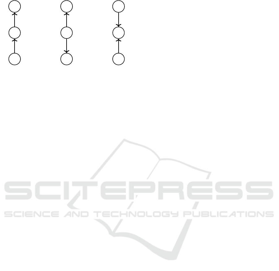
Figure 1: Possible three node DAGs. The structures 1b and

1a share the same set of independences therefore they be-

long to the same Markov class. The structure 1c are in a

different Markov class.

that share the same independence set (Glymour et al.,

2019; Spirtes, 2013). Figure 1 shows some possible

distributions with three variables. 1a entailed inde-

pendence between A and C given B (I(A, C|B)) and

1b also entailed I(A, C|B) that place it in the same

Markov Class. On the other hand, 1c entailed I(A, C)

and thus constitutes a different Markov Class.

Conventional approaches for discovering causal

structures rely on conditional independence proper-

ties, but there is another class of algorithms that com-

mits in search for a DAG best ﬁt the joint distribu-

tion. These methods may not use any of those inde-

pendence proprieties and yet lead to good results.

2.2.1 Constraint-based algorithms

These algorithms discover DAGs by testing the inde-

pendence between variables and adding (or removing)

edges based on these results. The PC (Spirtes et al.,

2000; Glymour et al., 2019) is the most known algo-

rithm of this class and represents a Bayesian network

as a set of independences. At ﬁrst, given the data,

the algorithm ﬁrst creates a complete graph in which

each node is a variable, which means an empty set of

independencies. For each round of the algorithm, all

combinations of nodes are tested for conditional inde-

pendence in the form I(X, Y |Z), with conditional set

Z starting from |Z| = 0 and adding 1 for the round.

For positive results in an independent test, the edge

between X and Y is removed and the set Z is saved in

association with the edge removed. When |Z| is less

than the DAG maximum degree, the independent test-

ing process stops and the sets Z are used to orient the

edges.

Since conditional independence relationships

presents symmetric aspects, the orientation round can

only obtain the Markov equivalence class of DAGs

(Kuipers et al., 2022).

The Conditional independence test adopted by the

algorithm has major impact in quality of obtained

structure and it may vary if the random variable is

continuous or discrete. Some commonly employed

conditional independence tests are Pearson’s correla-

tion (Baba et al., 2004) for continuous data, χ

test for

categorical data (Spirtes et al., 2000) and yet some

likelihood-based tests for all types of data (Tsagris

et al., 2018).

The estimating process of a conditional distribu-

tion Z for higher-order conditional independence tests

tends to deteriorate test results as long as |Z| in-

creases, especially for discrete variables with several

possible values. In fact, the number of sample sizes

needed to efﬁciently estimate the distribution grows

rapidly, leading to empty or nearly empty variable

cells (Spirtes et al., 2000).

2.2.2 Score-based Algorithms and Hybrid

Approaches

Unlike Constraint-based methods that rely on statisti-

cal proprieties and independence tests to achieve and

DAG on which to build the Bayesian network, score-

based algorithms settle the causal discovery problem

by using an evaluation method as a criterion to judge

whether a DAG candidate is good or not (Squires and

Uhler, 2022). Every DAG in the search space is a

possible solution; therefore, it becomes an optimiza-

tion problem based on a speciﬁc score method and a

sampler strategy for searching the DAG space (Koller

and Friedman, 2009).

2.2.3 Improved Physarum Learner

Inspired by the maze-solving ability of the slime mold

Physarum polycephalum, the Physarum Learner al-

gorithm was proposed adapting the Physarum Solver

capability of ﬁnding the optimal path in a maze

to the Bayesian network causal discovery problem

(Miyaji and Ohnishi, 2008). The Physarum-Maze is

formed by an initial fully connected graph with ran-

dom weights. In each Physarum Solver iteration, the

Source and Sink nodes are changed randomly, and the

weights are updated. Edges with weights above a cer-

tain threshold are marked as Bayesian network pos-

tulate edges, and then a score criterion deﬁnes if the

edge is kept or not in the ﬁnal network (Sch

on et al.,

2014).

An improved version of the Physarum Learner al-

gorithm was proposed in (Ribeiro et al., 2022). The

proposed implementation adds a search step, once a

new edge is inserted in the graph, for a conﬁguration

of reoriented edges that maximizes the score inside

a Markov class. Also, an extra procedure checks for

score stagnation, and if detected, the current iteration

is ﬁnished, minimizing time spent.

BIOSIGNALS 2023 - 16th International Conference on Bio-inspired Systems and Signal Processing

236

The evidence supports that Improved Physarum

Learner shows better computational performance

converging faster than the original method.

3 MATERIAL AND METHODS

In this section, descriptions are made to highlight

how the Pc Algorithm is combined with the Improved

Physarum Learner for solving the causal structure

learning problem, with the speciﬁcations of each step

and the validation methodology. In addition, the data

set and the ground truth structure are described. The

experiments were performed on a computer with the

following characteristics:

• Processor: Intel Core i5-10300H

• RAM: 16GB

• Operating System: Pop! OS 22.04 LTS

• Python: 3.8

• NumPy: 1.19.2

In its initial steps, Physarum Learner creates a

fully connected undirected graph called Physarum-

Maze. Data variables are nodes in the maze and each

edge has a weight randomly sampled from a uniform

distribution weight ∼ uniform[0.78, 0.79] that repre-

sents the impact of that edge on a Bayesian scoring

function. The Physarum Learner proposes to trans-

form the Physarum-Maze (a fully-undirected graph)

into a Bayesian Network (a directed acyclic graph) by

removing edges with an impact lower than a thresh-

old. Each edge weight is gradually updated using the

Physarum Solver output until it reaches stagnation,

which can be very time-consuming for large graphs.

The total number of Physarum Solver iterations is ap-

proximately n

, where n is the number of nodes in the

maze.

We believe that the process of updating edge

weights, already optimized in Improved Physarum

Learner, can take advantage of the use of a constraint

algorithm like the PC to further improve its perfor-

mance, especially in sparse graphs, which is where

the PC algorithm demonstrates its best results.

Both algorithms start with a similar structure and

then evaluate the effectiveness of each edge using dif-

ferent strategies. The independence tests in the PC

algorithm run faster than the estimation used in Im-

proved Physarum Learner, but it also leads to less pre-

cise results.

The idea is to modify the edge sampling distribu-

tion in the Physarum-Maze accordingly to the exis-

tence or not of that edge in the PC algorithm output,

expecting to accelerate the convergence process of

the Physarum-Maze edge weights. The base code for

the implementation of the PC algorithm was adapted

from (Callan, 2018) coupled with the χ

indepen-

dence test.

First, the PC algorithm is performed with the max-

imum order for the independence test equal to 1.

Then, Physarum-Maze structure are initialized, and

the edge weights are sampled as follows:

W (e) ∼

(

uniform[0.68 , 0.79], if e ∃ in PC output

uniform[0.28 , 0.39], otherwise

(3)

Where W (e) in Equation 3 is a sampling func-

tion that attributes a weight to edge e. In this case,

all edges preserved by the PC algorithm start with a

higher probability of existence in the ﬁnal structure.

A popular metric to test the performance of causal

discovery algorithms is to check the difference be-

tween the resulting graph structure and a known

ground-truth graph used to generate the dataset.

The LUng CAncer Simple set (LUCAS) (Guyon,

2022) is a popular dataset for learning causal graphs

and will be used in this work in addition to the Struc-

tural Hamming Distance (SHD) as a graph distance-

based metric (Cheng et al., 2022).

Lung Cancer

Smoking

Genetics

Anxiety

Peer Pressure

Yellow Fingers

Attention Disorder

Car Accident

Allergy

Coughing

Fatigue

Born an Even Day

Figure 2: Original LUng CAncer Simple set (LUCAS)

structure extracted from (Guyon, 2022). This structure was

artiﬁcially designed to model a Lung Cancer medical ap-

plication. It represents the statistical relationship between

behavioral and genetic variable in the likelihood of devel-

oping cancer in humans. Illustrate causes and possible con-

sequences.

LUCAS is an artiﬁcial dataset in which samples

are generated from a Bayesian network that represents

a medical application to diagnose, prevent and cure

lung cancer. All variables are listed in Table 1. Vari-

ables are divided into three main groups based on the

number of parents. Anxiety, Peer Pressure, Genetics,

Allergy and Born an Even Day are marked cyan and

do not have parents, for that reason they are not inﬂu-

enced by any other variable. In magenta are Yellow

Fingers and Attention Disorder which have Smoking

and Genetics as nodes with edges connecting to them,

respectively. And ﬁnally, in yellow, we have Smok-

ing inﬂuenced by Peer Pressure and Anxiety, Lung

cancer with edges coming from Smoking and Genet-

ics, Coughing with edges coming from Allergy and

Lung cancer, Fatigue inﬂuenced by Lung cancer and

Hybrid Improved Physarum Learner for Structure Causal Discovery

237

Coughing, and the last variable is Car accident with

Attention disorder and Fatigue as parent variables.

The subscript letter

after the variable name in

Table 1 represents the assumed value for the variables

corresponding to the respective probability shown in

the last column. From the data in Table 1 is possible

to marginalize all conditional probability tables by ex-

ploiting the fact that each entry in the conditional dis-

tribution must have a sum of 1 for a ﬁxed value of its

parents: for example, from the last line in Table 1 we

know that P(CarAccident = T |AttentionDisorder =

T, Fatigue = T ) = 0.97169 then we can com-

pute that P(CarAccident = F|AttentionDisorder =

T, Fatigue = T ) = 1 − 0.97169 = 0.02831. The joint

distribution generated a dataset with 1 million sam-

ples and was used for the causal discovery task.

Table 1: The Joint Probability Distribution for LUCAS

dataset. First column contain variable names, second col-

umn has variable parents (if exists) and the their current

state necessary for observe the conditional probability de-

scribed in column three. The Cyan rows represents vari-

ables without parents. In Magenta, the random variables

with one parent and the Yellow rows represents the nodes

with two parents.

Variable Parents Probability

Anxiety

0.64277

PeerPressure

0.32997

Genetics

0.15953

Allergy

0.32841

BornanEvenDay

0.5

YellowFingers

Smoking

0.23119

YellowFingers

Smoking

0.95372

AttentionDisorder

Genetics

0.28956

AttentionDisorder

Genetics

0.68706

Smoking

PeerPressure

, Anxiety

0.43118

Smoking

PeerPressure

, Anxiety

0.74591

Smoking

PeerPressure

, Anxiety

0.8686

Smoking

PeerPressure

, Anxiety

0.91576

Lungcancer

Genetics

, Smoking

0.23146

Lungcancer

Genetics

, Smoking

0.86996

Lungcancer

Genetics

, Smoking

0.83934

Lungcancer

Genetics

, Smoking

0.99351

Coughing

Allergy

, Lungcancer

0.1347

Coughing

Allergy

, Lungcancer

0.64592

Coughing

Allergy

, Lungcancer

0.7664

Coughing

Allergy

, Lungcancer

0.99947

Fatigue

Lungcancer

, Coughing

0.35212

Fatigue

Lungcancer

, Coughing

0.56514

Fatigue

Lungcancer

, Coughing

0.80016

Fatigue

Lungcancer

, Coughing

0.89589

CarAccident

AttentionDisorder

, Fatigue

0.2274

CarAccident

AttentionDisorder

, Fatigue

0.779

CarAccident

AttentionDisorder

, Fatigue

0.78861

CarAccident

AttentionDisorder

, Fatigue

0.97169

Figure 2 shows the graph structure of the 12 binary

random variables and their edges dependencies.

4 RESULTS AND DISCUSSION

In this section, relevant details for the LUCAS causal

structure are given, which include isolated variables

and their impact on the causal discovery problem.

The ﬁnal structure obtained from the proposed hybrid

methodology is also presented in this section in ad-

dition to the intermediate structure learned from PC

algorithm.

One characteristic of the structure of the LUCAS

network is the variable Born an Even Day that mea-

sures the impact of the day of birth on the chances of

developing lung cancer and, as expressed in Figure 2,

that the inﬂuence is negligible once there are no con-

nections with the rest of the DAG structure and, as a

consequence, should not inﬂuence any of the other 11

variables.

Identifying isolated variables is extremely impor-

tant once they have an irrelevant impact on tasks such

as forecasting or inference. In this case, the difference

between the search space for DAGs with 12 variables,

like LUCAS, has 5.2 × 10

more elements than the

search space for DAGs with 11 variables. So, it is

crucial that the statistical independence veriﬁcation

of the PC algorithm detects the Born an Even Day

isolated node from LUCAS and avoid the Improved

Physarum Learner from searching for irrelevant paths.

For that reason, different conditional indepen-

dence tests were performed and the χ

was selected

for PC algorithm execution. The experiment also

counted with Pearson Correlation (Hemmings and

Hopkins, 2006) and Fast Conditional Independence

Test (Chalupka, 2022).

Lung Cancer

Smoking

Genetics

Anxiety

Peer Pressure

Yellow Fingers

Attention Disorder

Car Accident

Allergy

Coughing

Fatigue

Born an Even Day

Figure 3: The PC algorithm obtained structure. In black are

the edges were preserved by the algorithm that are present in

the ground-truth structure. In green are the edges wrongly

kept by the algorithm. It has SHD = 7.

Figure 3 shows the structure obtained from the ex-

ecution of the PC Algorithm. The black edges are

the true positive edges kept by the algorithm that be-

longs to the ground truth graph, and all the edges of

the ground truth are present in the output of the PC

algorithm. The edge between Genetics and Attention

Disorder has arrowheads at each endpoint, showing

ambiguity in determining the direction of the edge

using the PC Algorithm. In addition, the algorithm

has truly isolated the variable Born an Even Day re-

BIOSIGNALS 2023 - 16th International Conference on Bio-inspired Systems and Signal Processing

238

ducing the chances of the improved Physarum learner

connecting it to anything else.

Lung Cancer

Smoking

Genetics

Anxiety

Peer Pressure

Yellow Fingers

Attention Disorder

Car Accident

Allergy

Coughing

Fatigue

Born an Even Day

Figure 4: The obtained structure from hybrid approach. In

black are the edges were preserved by the algorithm that are

present in the ground-truth structure. The green edge from

Attention Disorder to Genetics has reverse orientation. It

has SHD = 1.

Based on his partial result, the edge weights were

sampled as mentioned in section 3 as a starting point

for Improved Physarum Learner. Figure 4 shows the

learned structure that has SHD = 1. The only edge in-

correctly oriented from Attention Disorder to Genet-

ics is the same edge in which the PC algorithm had

difﬁculty determining the orientation. Despite that,

all edges kept by the Improved Physarum Learner be-

long to the ground-truth graph.

No major difference between the structure learned

by the methodology proposed in this work and the Im-

proved Physarum Learner, however, the hybrid ver-

sion presented a decrease in computational time. In

10 executions, the Improved Learner had an average

217.2 seconds to ﬁnd a structure, while the hybrid

had an average of 155.3 seconds, showing a consis-

tent 28% of time savings.

5 CONCLUSIONS

In this work, we presented a hybrid alternative for

Improved Physarum Learner in which we tested the

quality of the founded causal structure proposed in

(Guyon, 2022) by counting the Structural Hamming

Distance (SHD) between the learned structure and the

ground-truth graph. We also measured the computa-

tional time saved by adding information from Condi-

tional Independence tests into the Physarum maze.

The results showed consistency in the causal dis-

covery of the true structure with almost no errors.

The SHD = 1 refers to the green edge between Ge-

netics and Attention Disorder misoriented. In our

tests, the proposed methodology outperforms Im-

proved Physarum Learner, ﬁnding the causal struc-

ture on average 28% faster.

Although promising, the proposed combination of

algorithms needs, in future works, to be compared

with strategies of learning structures, both algorithms

consolidated in the literature and new approaches, us-

ing the same hardware and the same amounts of data

for all algorithms. Also, it is important to check the

Hybrid Improved Physarum behavior in different sce-

narios such as non-binary data, networks with a large

number of nodes, or even how it behaves with scarce

samples.

Furthermore, parallel implementation strategies

can be highly beneﬁcial for the Hybrid Improved

Physarum Learner. For the PC algorithm, the method-

ology proposed by (Le et al., 2016) seems promising

especially in high-dimensional data. But no parallel

technique was found by the authors relating causal

discovery problem and Physarum.

ACKNOWLEDGEMENTS

This work was partially supported by the follow-

ing agencies: CAPES, FAPESP 2014/50851-0, CNPq

465755/2014-3 and BPE Fapesp 2018/19150-6.

REFERENCES

Baba, K., Shibata, R., and Sibuya, M. (2004). Partial corre-

lation and conditional correlation as measures of con-

ditional independence. Australian & New Zealand

Journal of Statistics, 46(4):657–664.

Callan, J. (2018). Learning Causal Networks in Python.

Master’s thesis, University of York, England.

Chalupka, K. (2022). A fast conditional independence test

(fcit). https://github.com/kjchalup/fcit.

Cheng, L., Guo, R., Moraffah, R., Sheth, P., Candan, K. S.,

and Liu, H. (2022). Evaluation methods and measures

for causal learning algorithms. IEEE Transactions on

Artiﬁcial Intelligence.

Chickering, D. M. (2002). Optimal structure identiﬁcation

with greedy search. Journal of machine learning re-

search, 3(Nov):507–554.

Gasse, M., Aussem, A., and Elghazel, H. (2014). A hy-

brid algorithm for bayesian network structure learn-

ing with application to multi-label learning. Expert

Systems with Applications, 41(15):6755–6772.

Glymour, C., Zhang, K., and Spirtes, P. (2019). Review of

causal discovery methods based on graphical models.

Frontiers in genetics, 10:524.

Guo, R., Cheng, L., Li, J., Hahn, P. R., and Liu, H. (2020).

A survey of learning causality with data: Problems

and methods. ACM Computing Surveys (CSUR),

53(4):1–37.

Guyon, I. (2022). Causality workbench project.

http://www.causality.inf.ethz.ch/data/LUCAS.html.

Hemmings, H. C. and Hopkins, P. M. (2006). Foundations

of anesthesia: basic sciences for clinical practice. El-

sevier Health Sciences.

Hybrid Improved Physarum Learner for Structure Causal Discovery

239

Huang, J. and Zhou, Q. (2022). Partitioned hybrid learning

of bayesian network structures. Machine Learning,

pages 1–44.

Koller, D. and Friedman, N. (2009). Probabilistic graphical

models: principles and techniques. MIT press.

Kuipers, J., Suter, P., and Moffa, G. (2022). Efﬁcient

sampling and structure learning of bayesian networks.

Journal of Computational and Graphical Statistics,

pages 1–12.

Le, T. D., Hoang, T., Li, J., Liu, L., Liu, H., and Hu,

S. (2016). A fast pc algorithm for high dimensional

causal discovery with multi-core pcs. IEEE/ACM

transactions on computational biology and bioinfor-

matics, 16(5):1483–1495.

Meek, C. (2013). Causal inference and causal expla-

nation with background knowledge. arXiv preprint

arXiv:1302.4972.

Miyaji, T. and Ohnishi, I. (2008). Physarum can solve the

shortest path problem on riemannian surface mathe-

matically rigourously. International Journal of Pure

and Applied Mathematics, 47(3):353–369.

Nandy, P., Hauser, A., and Maathuis, M. H. (2018).

High-dimensional consistency in score-based and hy-

brid structure learning. The Annals of Statistics,

46(6A):3151–3183.

Neapolitan, R. E. et al. (2004). Learning bayesian networks,

volume 38. Pearson Prentice Hall Upper Saddle River.

Pearl, J. (2018). Theoretical impediments to machine learn-

ing with seven sparks from the causal revolution.

arXiv preprint arXiv:1801.04016.

Ribeiro, V. P., RP, B., Maciel, C. D., and Balestieri,

J. A. (2022). An improved bayesian network super-

structure evaluation using physarum polycephalum

bio-inspiration. In Congresso Brasileiro de Au-

tom

atica-CBA, volume 2.

Sch

on, T., Stetter, M., Tom

e, A. M., Puntonet, C. G., and

Lang, E. W. (2014). Physarum learner: A bio-inspired

way of learning structure from data. Expert systems

with applications, 41(11):5353–5370.

Spirtes, P. and Glymour, C. (1991). An algorithm for fast

recovery of sparse causal graphs. Social science com-

puter review, 9(1):62–72.

Spirtes, P., Glymour, C. N., Scheines, R., and Heckerman,

D. (2000). Causation, prediction, and search. MIT

press.

Spirtes, P. L. (2013). Directed cyclic graphical rep-

resentations of feedback models. arXiv preprint

arXiv:1302.4982.

Squires, C. and Uhler, C. (2022). Causal structure learn-

ing: a combinatorial perspective. arXiv preprint

arXiv:2206.01152.

Tank, A., Covert, I., Foti, N., Shojaie, A., and Fox, E. B.

(2021). Neural granger causality. IEEE Transac-

tions on Pattern Analysis and Machine Intelligence,

44(8):4267–4279.

Tsagris, M., Borboudakis, G., Lagani, V., and Tsamardi-

nos, I. (2018). Constraint-based causal discovery with

mixed data. International journal of data science and

analytics, 6(1):19–30.

Tsamardinos, I., Brown, L. E., and Aliferis, C. F. (2006).

The max-min hill-climbing bayesian network struc-

ture learning algorithm. Machine learning, 65(1):31–

78.

BIOSIGNALS 2023 - 16th International Conference on Bio-inspired Systems and Signal Processing

240