VoronoiPatches: Evaluating a New Data Augmentation Method

Steffen Illium, Gretchen Grifﬁn, Michael K

olle, Maximilian Zorn, Jonas N

ußlein

and Claudia Linnhoff-Popien

Institute of Informatics, LMU Munich, Oettingenstraße 67, Munich, Germany

ﬁ

Keywords:

Voronoi Patches, Information Transport, Image Classiﬁcation, Data Augmentation, Deep Learning.

Abstract:

Overﬁtting is a problem in Convolutional Neural Networks (CNN) that causes poor generalization of models

on unseen data. To remediate this problem, many new and diverse data augmentation (DA) methods have

been proposed to supplement or generate more training data, and thereby increase its quality. In this work,

we propose a new DA algorithm: VoronoiPatches (VP). We primarily utilize non-linear re-combination of

information within an image, fragmenting and occluding small information patches. Unlike other DA methods,

VP uses small convex polygon-shaped patches in a random layout to transport information around within an

image. In our experiments, VP outperformed current DA methods regarding model variance and overﬁtting

tendencies. We demonstrate DA utilizing non-linear re-combination of information within images, and non-

orthogonal shapes and structures improves CNN model robustness on unseen data.

1 INTRODUCTION

Fueled by big data and the availability of powerful

hardware, deep Artiﬁcial Neural Networks (ANNs)

have achieved remarkable performance in computer

vision thanks to recent advancements. But deeper

and wider networks with more and more parameters

are data hungry beasts. (Aggarwal, 2018) With these

(often oversized) ANNs a sufﬁcient amount of train-

ing data is critical for good performance and avoiding

overﬁtting for a wide variety of problems. Unfortu-

nately, data sources can be difﬁcult to appropriately

work with due to mistakes made while acquiring data,

mislabeling, underrepresentation, imbalanced classes,

et cetera (Illium et al., 2021; Illium et al., 2020). In

these cases, learning directly from real-world datasets

may not be straightforward. To overcome this chal-

lenge, Data Augmentation (DA) is commonly used

because of its effectiveness and ease of use (Shorten

and Khoshgoftaar, 2019). Over the years, various

methods (e.g., occlusion, re-combination, fragmenta-

tion) have been developed, reviewed and contrasted.

In this work, we propose a logical combination of

such existing DA-methods: VoronoiPatches (VP).

First, we introduce the concept of DA and Voronoi

diagrams in section 2. A discussion of existing, re-

lated works follows in section 3. We propose our ap-

proach (VP), dataset, and experimental setup and re-

sults in section 4. Finally, we summarize our ﬁndings

and give an outlook for future research in section 5.

2 PRELIMINARIES

Data Augmentation (DA) is a technique used to re-

duce overﬁtting in ANNs, which in the most extreme

cases has perfectly memorized its training data; and

is therefore, unable to generalize well (the major ad-

vantage of ANNs). A function learned by an overﬁt

model exhibits high variance in its output (Shorten

and Khoshgoftaar, 2019) by overestimating, which

ultimately leads to poor overall performance. The

amount of a model’s variance can be thought of as

a function of its size. Assuming ﬁnite samples, the

variance of a model will increase as its number of pa-

rameters increases. (Burnham and Anderson, 2002)

This is where DA methods can be applied (on training

data) to increase the size and diversity of an otherwise

limited (e.g., size, balance) dataset.

In the past and with the advent of deep CNN,

such approaches have been very successful in the do-

main of computer vision (and many others) (Shorten

and Khoshgoftaar, 2019). Image data is especially

well suited for augmentation, as one major task of

ANNs is being robust to object invariance and image

features.DA algorithms, on the other hand, are made

to generate such invariances. We restrict our discus-

sion to image data as many other comparable domains

exhibit their own challenges and characteristics.

Generally, a dataset supplemented with aug-

mented data represents a more complete set of all

possible data, i.e., it closes the real-world gap and

350

Illium, S., Grifﬁn, G., Kölle, M., Zorn, M., Nüßlein, J. and Linnhoff-Popien, C.

VoronoiPatches: Evaluating a New Data Augmentation Method.

DOI: 10.5220/0011670000003393

In Proceedings of the 15th International Conference on Agents and Artiﬁcial Intelligence (ICAART 2023) - Volume 3, pages 350-357

ISBN: 978-989-758-623-1; ISSN: 2184-433X

 2023 by SCITEPRESS – Science and Technology Publications, Lda. Under CC license (CC BY-NC-ND 4.0)

promotes the ability to generalize. Data warping

methods transform existing data to inﬂate the size of

a dataset, whereas oversampling methods synthesize

entirely new data to add to a dataset (Shorten and

Khoshgoftaar, 2019).

Voronoi diagrams are geometrical structures which

deﬁne the partition of a space using a ﬁnite set of

distinct and isolated points (generator points). Every

other point in the space belongs to the closest gener-

ator point. Thus, the points belonging to each gen-

erator point form the regions of a Voronoi diagram.

(Okabe et al., 2000) In the following, we focus on

2-dimensional Voronoi diagrams (spanning Euclidean

space), as used in this work.

Let S be a set of n ≥ 3 generator points p, q, r . . .

in Euclidean space R

. The distance d between an

arbitrary point x = (x

, x

) and the generator point p =

, p

) is given as:

d(p, x) =

− x

)

+ (p

− x

)

(1)

If we examine generator points p and q, we can

deﬁne a line which is mutually equidistant as:

D(p, q) = {x|d(p, x) ≤ d(q, x)} (2)

A Voronoi region belonging to a generator point

p ∈ S, V R(p, S), is the intersection of half-planes

D(p, q) where q ranges over all p in S:

V R(p, S) =

q∈S,q̸=p

D(p, q) (3)

In other words, Voronoi region of p (V R(p, S)) is

made up of all points x ∈ R

for which p is the near-

est neighboring generator point. This results in a con-

vex polygon, which may be bounded or unbounded.

The boundaries of regions are called edges, which are

constrained by their endpoints (vertices). An edge be-

longs to two regions; all points on an edge are clos-

est to exactly two generator points. Vertices are sin-

gle points that are closest to three or more generator

points. Thus, the regions of a Voronoi diagram form

a polygonal partition of the plane, V (P). (Aurenham-

mer, 1991; Aurenhammer et al., 2013)

3 RELATED WORK

With the preliminaries introduced, we now survey

some existing and related work from the ﬁeld of Data

Augmentation in the context of deep Artiﬁcial Neural

Networks.

3.1 Occlusion

Methods employing the principle of occlusion mask

parts of model input. Consequentially, a model en-

counters more varied combinations of an object’s fea-

tures and context forcing stronger recognition of an

object by its structure. Two of the earliest methods

that use occlusion are Cutout (Devries and Taylor,

2017) and Random Erasing (RE) (Zhong et al., 2017).

Both remove one large, contiguous region from train-

ing images (cf. Figure 1, 1A-B). Through Hide-and-

Seek (HaS) Neural Networks (NNs) learn to focus on

the overall object, occluding parts of the input (Singh

et al., 2018). This approach removes more varied

combinations of smaller regions in a grid pattern from

neighboring model input (cf. Figure 1, 3C, 4A). How-

ever, removed regions may also form a larger contigu-

ous region which may lead to the removal of all of an

object (or none of it), which is the same major limi-

tation of early DA methods. GridMask (Chen et al.,

2020) tries to prevent these two extremes by removing

uniformly distributed regions (cf. Figure 1, 1C, 2A).

While the use of simple orthogonal shapes and

patterns is a common characteristic of occlusion-

based methods, Voronoi decomposition-based ran-

dom region erasing (VDRRE) demonstrates a po-

tential advantage of removing more complex shapes

(Abayomi-Alli et al., 2021). For the tasks of facial

palsy detection and classiﬁcation, VDRRE evaluated

the use of Voronoi tessellations (cf. Figure1, 3A-B).

An additional choice of many regional dropout

methods is the color of the occlusion mask. Op-

tions include random values, the mean pixel value

of the dataset, or black or white pixels (Yun et al.,

2019). Relevant literature includes (Devries and Tay-

lor, 2017; Zhong et al., 2017; Chen et al., 2020;

Singh et al., 2018; Abayomi-Alli et al., 2021). Fur-

thermore, regional dropout methods are not always

label-preserving, depending on the dataset (Shorten

and Khoshgoftaar, 2019).

3.2 Re-Combination of Data

DA methods which re-combine data, mix training im-

ages (non-)linearly. This has been found to be an ef-

ﬁcient use of training pixels (over regional dropout

methods) (Yun et al., 2019), in addition to increas-

ing the variety of dataset samples (Takahashi et al.,

2018). However, mixed images do not necessarily

make sense to a person (Shorten and Khoshgoftaar,

2019) (e.g., lower section in Figure 1, 4A-B + Row 5)

and it is not fully understood why mixing images in-

creases performance (Summers and Dinneen, 2018).

Non-linear mixing methods combine parts of im-

ages spatially. CutMix (Yun et al., 2019) and Random

image cropping and pasting (RICAP) (Takahashi

et al., 2018) are non-linear methods that combine

parts of two or four training images, respectively.

VoronoiPatches: Evaluating a New Data Augmentation Method

351

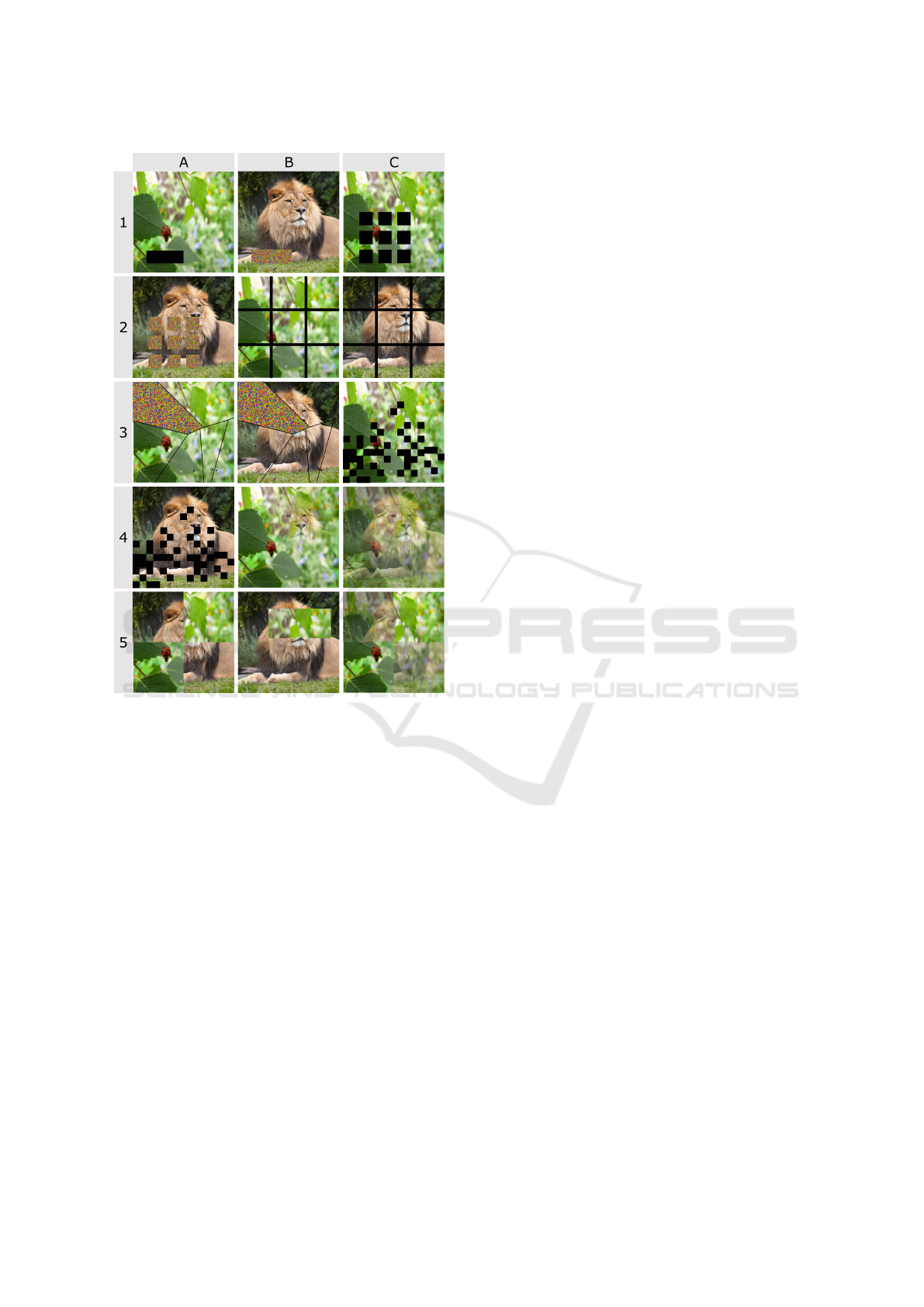
Figure 1: Combined Augmentations Showcase: Overview

of some DA methods. Rows 1-3 + 4A: Occlusion methods;

4B-C + Row 5: (Non-) Linear combination methods.

Corresponding labels are mixed proportionately to the

area of each image used. CutMix ﬁlls a removed re-

gion with a patch cut from the same location in an-

other training image (cf. Figure 1, 5B) (Yun et al.,

2019). RIACP combines four images in a two by two

grid (Takahashi et al., 2018).

Linear mixing methods combine two images by

averaging their pixels (Shorten and Khoshgoftaar,

2019). There are several methods that use this

approach, including Mixup (Zhang et al., 2017),

Between-class Learning (Tokozume et al., 2017), and

SamplePairing (Inoue, 2018) (cf. Figure 1, 4B-C,5C).

(Inoue, 2018) found mixing images across the entire

dataset produced better results than mixing images

within classes. Although mixed images may not make

semantic sense, they are surprisingly effective at im-

proving model performance (Summers and Dinneen,

2018). A critique on how linear methods introduce

“unnatural artifacts”, which may confuse a model, can

be found in (Yun et al., 2019).

3.3 Fragmentation

Fragmentation may occur as a side effect of pixel

artifacts introduced by occlusions (Lee et al., 2020)

or non-linear mixing of images (Takahashi et al.,

2018), which create sudden transitions at the edges

of removed regions or combined images, respectively.

While occluding and mixing information may pre-

vent the network from focusing on easy characteris-

tics, deep ANNs may also latch on to boundaries cre-

ated by these pixel artifacts.

In SmoothMix (Lee et al., 2020) the transition be-

tween two blended images is softened to deter the net-

work from latching on to them. Alpha-value masks

with smooth transitions are applied to two images,

which are then combined. Furthermore, Smooth-

Mix prevents the network behavior of focusing on

“strong-edges” and achieves improved performance

while building on earlier image blending methods like

CutMix.

Cut, Paste and Learn (CPL) (Dwibedi et al., 2017)

is a DA method developed for instance detection. To

create novel, sufﬁciently realistic training images, ob-

jects are pasted on random backgrounds while the ob-

ject’s edges are either blended or blurred. Although

the resulting images look imperfect to the human eye,

they perform better than manually created images or

training on real data alone (Dwibedi et al., 2017).

While SmoothMix and CPL aim to minimize arti-

ﬁcially introduced boundaries, MeshCut (Jiang et al.,

2020) uses a grid-shaped mask to fragment informa-

tion in training images and purposefully introduces

boundaries within an image (cf. Figure 1, 2B-C). By

doing so, the model learns an object by its many

smaller parts, thereby focusing on broader areas of

an object. In contrast to SmoothMix and CPL, Mesh-

Cut demonstrates that intentionally created bound-

aries can improve model performance.

4 METHOD

Noticing the beneﬁts of using non-trivial edges in-

troduced by randomly organized Voronoi diagrams

(Abayomi-Alli et al., 2021), as well as the power of

occluding multiple small squares (HaS)(Singh et al.,

2018), we opted for a conceptional fusion of these ap-

proaches. From our perspective, there also is the need

for a DA technique which does not occlude wide areas

of the image (that may hold the main features), as the

occlusion of areas with black (zero-values) or Gaus-

sian noise seems to not be fully error-free. There-

fore, we argue in favor of a new category of Data

Augmentation methods: Transport. The main idea

ICAART 2023 - 15th International Conference on Agents and Artiﬁcial Intelligence

352

of transport-based approaches is to preserve features

and reposition them in their natural context, in con-

trast to a replacement by non-informative data. Com-

bined with the concept of non-trivial edges (Voronoi

diagram) and occlusion-of-many HaS, we suggest

VoronoiPatches (VP).

4.1 VoronoiPatches (VP)

Our goal was to supplement training data using novel

images generated online through a non-linear trans-

formation. To do so, an image is partitioned into a

set of convex polygons (patches) using a Voronoi di-

agram. A ﬁxed number of patches are randomly cho-

sen and copied from the original image. Then, these

are pasted randomly over the center of a polygonal

region (cf. Figure 2). The result is a (novel) image

containing (mostly) the same object features. VP may

occlude and duplicate parts of the object in the orig-

inal image while preserving the original label. The

location, number, and visibility of an object’s parts

in an image vary each time VP is applied. By re-

combining information within the image instead of

replacing them with random values or a single value,

information loss is minimized. Due to the random

nature of a patch’s shape, size, and ﬁnal location,

patches may overlap or not move at all. This proce-

dure is further described in algorithm 1.

There are three tunable Hyperparameters (HPs):

Number of generator points: The approximate size

and number of patches generated by a Voronoi par-

tition. Using few generator points results in fewer

larger polygons, and v.v. Number of patches: The

number of patches to be transported. Smooth: The

transition style between moved patches and the orig-

inal image. This may be left as they are (sudden)

or smoothed. Sudden transitions may create pixel

artifacts caused by sudden changes in pixel values,

whereas the application of smooth transitions reduces

this effect (cf. Figure 3).

4.2 Setup & Dataset

In this section, we brieﬂy outline our data pipeline and

introduce the dataset and performance metrics used.

First, we use an 85:15 split of our training set as an

additional validation set for model selection. During

the training process, performance metrics were calcu-

lated and collected each epoch on both the training

and validation sets and used to monitor the training

process. Measurements were based on the checkpoint

with the highest measured accuracy; we note that this

may over- or underestimate true performance (Aggar-

wal, 2018).

Algorithm 1: VoronoiPatches.

Input : sample, generators, patches, smooth

Output: aug

begin:

aug ← copy of sample

polygons ← Voronoi(generators);

centroids ← [mean(p) in polygons];

for range(patches) do

p ← random(polygons);

c ← random(centroids);

Move p such that arith.Mean(p) = c;

for x, y in p do

aug[x, y] ← sample[x, y];

if smooth then

s ← gauss.Filter(aug);

borders ← calc border();

for xy

in borders do

aug[xy

] ← s[xy

];

The dataset was chosen based on two factors:

sample size and dataset size. By using medium to

large resolution images, we ensure more variation in

partitions computed and the ability to generate small

enough polygons.

The 2012 ImageNet Large-Scale Visual Recogni-

tion Challenge (ILSVRC) dataset

, colloquially re-

ferred to as ImageNet, consists of 1.2 million train-

ing and 60,000 validation full-resolution images cat-

egorized and labeled according to a WordNet

based

class hierarchy into 1,000 classes (Russakovsky et al.,

2015). While the images’ resolution is sufﬁcient, the

size of the dataset in its entirety is impractical for our

experiments.

We used the “mixed 10” dataset(Engstrom et al.,

2019), which is a subset of the 2012 ImageNet

dataset.

As “mixed 10” is a well-balanced dataset, we

chose the performance metric classiﬁcation accuracy

in %. Additionally, we examined the variance and en-

tropy introduced by the DA methods.

4.3 Experimental Setup

Baseline. We ﬁrst established a baseline model

based on SqueezeNet 1.0 (through grid search), which

provides us with default performance metrics. We

chose SqueezeNet 1.0 because it was designed specif-

ically for multi-class image classiﬁcation using Im-

ageNet and has a small parameter footprint (Ian-

dola et al., 2016). Using 50x fewer parameters, it

matched or outperformed the top-1 and top-5 accu-

racy (Iandola et al., 2016) of the 2012 ILSVRC win-

http://www.image-net.org/

https://wordnet.princeton.edu/

VoronoiPatches: Evaluating a New Data Augmentation Method

353

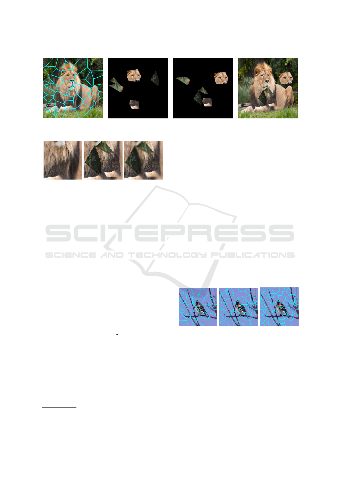
Figure 2: VP: An example image and its Voronoi diagram (50 generator points), 5 randomly selected patches copied, then

transported to random locations, and the resulting novel image with sudden transitions (left to right).

Figure 3: Voronoi Patches: The original image (left), the

same image augmented with sudden (middle), or smooth

transitions (right).

ner, AlexNet, which has approximately 60 million pa-

rameters (Krizhevsky et al., 2017).

We made one modiﬁcation to the original net-

work architecture by introducing a batch normaliza-

tion layer. This serves to normalize the distribution

of our training dataset in a batch-wise fashion. Since

DA is performed online, it is our only chance to do

so consistently across all models and DA methods.

Initial model HPs were adjusted in a “best guess ap-

proach” according to literature. There is no guarantee

that we found an optimal conﬁguration; however, our

goal was to set up an efﬁcient and well-functioning

model for evaluation.

Furthermore, we chose cross-entropy as a com-

mon multi-class classiﬁcation loss (Wang et al., 2022)

and ADAM (Kingma and Ba, 2014) as optimizer,

which uses adaptive learning rates that typically re-

quire less tuning and converge faster (Ruder, 2016).

Optimizer HPs: lr = 0.0001, betas = (0.9, 0.999),

and eps = 1e − 08 with batch size = 32. As the

SqueezeNet 1.0 architecture (using ReLU) requires

images at 224x224x3 (Iandola et al., 2016), we re-

sized to this resolution and scaled all images channel-

wise in the range of [0, 1] using min-max normaliza-

tion

. By completing this step, the pixel values of our

dataset have the same scale as the networks’ parame-

ters, which may improve convergence time by stabi-

lizing the training procedure (Aggarwal, 2018). There

were no further transformations or augmentations for

the baseline model.

Scikit-learn/Preprocessing: Min-Max-Scale

Our choice of VoronoiPatches HPs was inﬂuenced

by the characteristics of our dataset and reﬂects the

two main goals: To preserve the label of each aug-

mented image and to occlude or repeat the features of

an object or its context in a distributed manner. The

diversity of samples in our dataset creates a challeng-

ing situation for choosing an optimal number of gen-

erator points. Speciﬁcally, the object-to-context ra-

tio can vary greatly. In an image where the object

is tiny, the danger of all features being occluded by

VP is still present. Given the variety of this ratio

in the “mixed 10” dataset, it is difﬁcult to estimate

what size patch might be too small or large, or how

many patches (i.e., total pixels

moved) are necessary

to have a positive impact on model performance. To

balance the parameter space of our grid search with

the variation in object-to-context ratio in our dataset,

we chose generators = {50, 70, 90}, cf. Figure 4. To

explore how the size and number of patches might

impact performance, we chose patches = {5, 10, 15}.

For all combinations, we also considered both transi-

tion styles, smooth = {true, f alse}.

Figure 4: Voronoi Diagrams: Computed with (left) 50,

(middle) 70, and (right) 90 generator points.

Reproducibility. To ensure the reproducibility of

our results, we seeded our interpreter environment,

as well as all random number generators involved in

the training process. All models (and DA methods)

along all grid searches use the same seed to ensure

reproducibility and validity. Seeds were chosen at

random from [0, 2

− 1]. To calculate the avg. ex-

pected performance, we re-trained our baseline model

with the best performing HP values with the afore-

mentioned seeded grid search. After training to con-

ICAART 2023 - 15th International Conference on Agents and Artiﬁcial Intelligence

354

Figure 5: 1: Train and val. accuracy (100 epochs); 2: CE-loss. Over-ﬁtting visible; 3: Avg. SSIM for VP and RE; 4: Avg.

effect of VP (dark blue=sudden, light blue=smooth transitions) and RE (gray lines) measured in entropy H.

vergence (100 epochs, max. acc. 80.1% at epoch

74), the highest accuracy checkpoints are selected for

each seed. To ﬁnd suitable VP HPs, we performed a

grid search over all combinations of generators and

patches, w/ and w/o smoothing. Predeﬁned by the

baseline model, the training of DA methods was lim-

ited to 100 epochs.

Results. For all numbers of patches and patch

sizes of VP used while training, we observed a per-

formance improvement over baseline performance.

While this improvement is clear, our results showed

this gain varies across HP combinations. The high-

est validation accuracy for VP that can be reported

is 83.6% with HPs: generators=70, patches=15, and

smooth=False. We observed an improvement in val.

acc. by about 1.3-3.5% over the baseline models

for all models trained with VP. On the test set (un-

seen in training and validation), we evaluated the

performance of the resulting best baseline and op-

timal VP models. The avg. expected performance

is 80.9% accuracy, 80.9% macro-recall, and 81%

macro-precision. The avg. expected performance of

a model trained using VP is 83.3% accuracy, 83.5%

macro-precision, and 83.3% macro-recall.

Even though macro-measures are quite similar,

the performance of individual classes varies as ex-

pected.

However, the classes Car and Truck both perform

about 10-30% worse than the others due to noisy la-

bels and for which ImageNet was recently strongly

critiqued (Beyer et al., 2020).

Smoothing. Unfortunately, we did not observe any

clear improvement in the performance of VP using

smooth over sudden transitions (smooth=false). The

best performing models use sudden transitions, based

on our observations in model training; however, we

cannot rule out a possible advantage at this time.

Dependent on the other HPs, either approach can

be of advantage. We implemented the width of the

smoothed transition between patch and image with

a ﬁxed factor. In future works, this could be intro-

duced as another HP. Both smoothing and the factor

could also be bound to a stochastic process (sampled

on each VP application).

Comparisons. To verify the validity and utility of

VP, we evaluated the performance of the RE, VDRRE

and a combination of both, using the same procedure

as outlined above. For RE HPs outlined in (Zhong

et al., 2017), black (0) and random (uniform [0,1))

pixel values were chosen. Figure 5: 1 shows an

avg. acc. improvement by VP over RE of 0.6%-

0.7%. VDRREs parameters were chosen as sug-

gested. (Abayomi-Alli et al., 2021) used six regions,

of which one was then occluded with noise. On our

dataset, VDRRE achieved results, which are close to

RE. MeshCut (augmentation schedule and HPs as

stated by (Jiang et al., 2020)) behaved worse than

‘Random’ VP. Inspired by the occlusion with Gaus-

sian noise, we also tested a VP version with randomly

ﬁlled patches, rather than transporting sections of the

image (more or less comparable with VDRRE, but at

smaller scale). ‘Random’ VP achieved better results

than both, VDRRE and RE, while performing close

to VP.

Entropy H. To measure the effect of our method

on the training data, we employed entropy H involv-

ing the resulting prob. distribution of each image x

(with P := prob., K := classes): H(x) = −

∑

kεK

P(k)∗

log(P(k)) (Goodfellow et al., 2016). We then aggre-

gated the entropy scores for all images with the arith-

metic mean (cf. Figure 5): 4. The avg. entropy is a

measure of how balanced the prob. distributions are

on avg. (Goodfellow et al., 2016). For a prob. dis-

tribution of 10 values (for 10 classes) the lower and

upper bounds for entropy are 0.00 and 3.32, respec-

tively. The bounds correspond to the case of a perfect

classiﬁcation with 1.0 probability for one class and

0.0 for all others (low entropy) and the case of per-

fectly balanced probability of 0.1 across all classes

(high entropy). As anticipated, the more data trans-

ported within an image by VP the more uncertainty

is embedded in the model’s output (i.e., the more bal-

anced the model’s prob. distributions are). We ob-

serve that this effect is greater among all VP HP com-

binations than RE with either black or random pixels.

We attribute the reduced entropy of RE using random

pixels over black pixels to the model ﬁnding patterns

in these values.

VoronoiPatches: Evaluating a New Data Augmentation Method

355

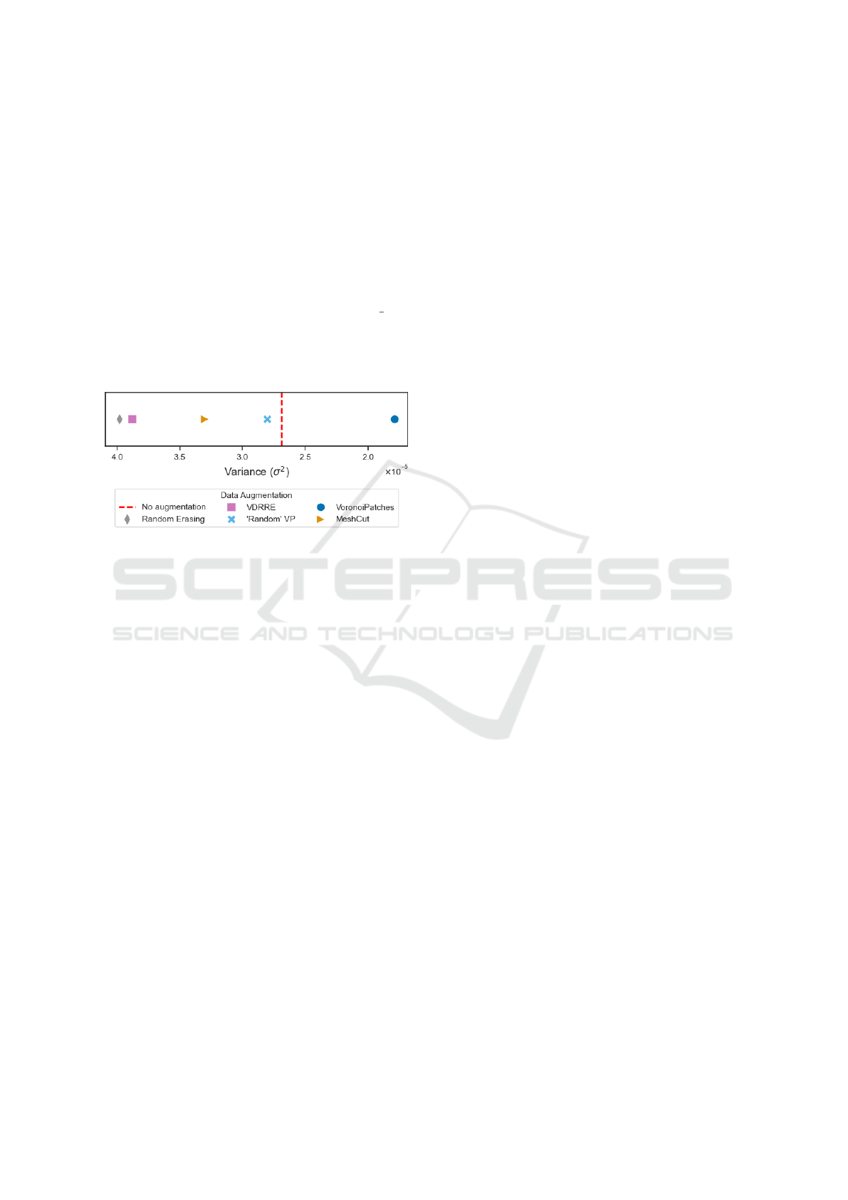
Main Findings. (1) Figure 6 shows the measured

variance for examined DA methods. Over all seeded

runs, our proposed method (VP) exhibits the lowest

variance, even lower than training on non-augmented

training data. Taking the results of the entropy analy-

sis (above) in to consideration, we found the last point

to be quite a surprising ﬁnding.

(2) By inspecting the avg. acc. and the CE-loss in Fig-

ure 5: 2 we observe an additional interesting ﬁnding.

All training runs (w/ and w/o DA) came at the cost

of still overﬁtting to the training data of “mixed 10”.

Our method VP, in contrast to all those compared,

showed the least amount of overﬁtting. This can be

observed in the growing distance of the CE-loss in

Figure 5: 2.

Figure 6: Model Variance Comparison Avg. test variance

(std) of VP and the other DA methods.

Further Analysis. The number of generator points

determines the avg. patch size. We collected the avg.

pixels

(2D area) for bounded polygons using 50, 70,

and 90 generator points. The avg. patch sizes are 932,

673, and 528 pixels

, respectively. We observe that

using many smaller patches (15 patches, 528 pixels

as well as using fewer larger patches (5 patches, 932

pixels

) results in better model performance on avg.

We observe no clear improvement using smooth tran-

sitions; we assume, either, that the transition areas’

width is not optimal or that the pixel artifacts have

a positive effect similar to the mesh mask in (Jiang

et al., 2020).

To measure how different HP values change our

images, we calculate the Structural SIMilarity In-

dex (SSIM) between orig. and augmented images.

SSIM was developed as a measurement ([0-1]) of

degradation by comparing the luminance, contrast,

and structures of two images (Wang et al., 2005).

SSIM(original, augmented) = 1.0 represents the triv-

ial case of a perfect match (identical images) (Wang

et al., 2005). Collecting and aggregating (arith. mean)

SSIM values for 1,000 iterations with several HP

combinations Figure 5 conﬁrmed that by increasing

the number of patches or decreasing the number of

generators, the SSIM of original and augmented im-

ages decreases. The relationship between the avg.

SSIM and avg. entropy is approximately linear. As

the structural difference in augmented images in-

creases, so does the entropy of the predictions for

these images.

Further, we observe a drop-off in performance

when more than approx. 10,000 total pixels

are

transported. The best performance was achieved

with 10,095 total pixels

(generators = 70, patches =

15, smooth = False), a re-combination of 20.1% of an

images’ data.

There appears to be an optimal avg. patch size

and/or number of patches moved similar to the op-

timal ratio of the grid mask of uniformly distributed

squares in (Chen et al., 2020), which controls how

many squares make up the mask, as well as how

much space masked between. As a point of reference,

the avg. rectangle size generated by Random Eras-

ing (RE) is 10,176 pixels

. In accordance with the

default values in (Zhong et al., 2017), RE was applied

with a probability of 50%. On avg., RE removes a

rectangle equal to 20.3% of an image when applied,

whereas VP re-orders patches equal to 20.1%, com-

bined, in each image.

We noticed an improvement in performance by

re-combining many small VP patches over randomly

erasing one large contiguous rectangle with 50%

probability (RE).

Variance in patch sizes is also determined by

how generator points are distributed across the image.

Through visual inspection, a trend of smaller patches

resulting from more generator points, and v.v., can be

observed.

5 CONCLUSION

In this work we introduced VoronoiPatches (VP), a

novel DA method, and data warping category (trans-

port) to solve the problem of overﬁtting for CNNs.

We sought to minimize information loss and pixel ar-

tifacts, as well as exploit non-orthogonal shapes and

structures in DA. Our method, which employs non-

orthogonal shapes and structures to re-combine infor-

mation within an image, outperforms the existing DA

methods regarding model variance and overﬁtting ten-

dencies. Additional experiments analyzed VP’s inﬂu-

ence on predictions, as well as the inﬂuence of HP

values on performance. We show that there are further

opportunities to build on our ﬁndings and add validity

to our initial evaluation of VP. This includes: opti-

mizing smooth transitions, exploring different pixel

values or patch shapes (to better understand the con-

tribution to DA), mixing images across the training

set, and eventually exploring applications of VP in

ICAART 2023 - 15th International Conference on Agents and Artiﬁcial Intelligence

356

other tasks or ﬁelds (e.g., medical image analysis or

the ﬁeld of audio in the form of mel spectrograms).

From a practical standpoint, solving the limitation of

expensive training would enable more efﬁcient usage

of the available datasets. Currently, expensive train-

ing is a limitation of VP, which is also a possible fu-

ture task.

REFERENCES

Abayomi-Alli, O. O., Dama

sevi

cius, R., Maskeli

unas, R.,

and Misra, S. (2021). Few-shot learning with a

novel voronoi tessellation-based image augmentation

method for facial palsy detection. Electronics, 10(8).

Aggarwal, C. C. (2018). Neural Networks and Deep Learn-

ing: A Textbook. Springer Publishing Company, In-

corporated, 1st edition.

Aurenhammer, F. (1991). Voronoi diagrams—a survey of a

fundamental geometric data structure. ACM Comput.

Surv., 23(3):345–405.

Aurenhammer, F., Klein, R., and Lee, D.-T. (2013). Voronoi

Diagrams and Delaunay Triangulations. World Sci-

entiﬁc Publishing Co., Inc., USA, 1st edition.

Beyer, L., H

enaff, O. J., Kolesnikov, A., Zhai, X., and Oord,

A. v. d. (2020). Are we done with imagenet? arXiv

preprint arXiv:2006.07159.

Burnham, K. P. and Anderson, D. R. (2002). Model

selection and multimodel inference : a practical

information-theoretic approach. Springer-Verlag,

New York, NY, 2nd edition.

Chen, P., Liu, S., Zhao, H., and Jia, J. (2020). Gridmask

data augmentation. CoRR, abs/2001.04086.

Devries, T. and Taylor, G. W. (2017). Improved regular-

ization of convolutional neural networks with cutout.

CoRR, abs/1708.04552.

Dwibedi, D., Misra, I., and Hebert, M. (2017). Cut, paste

and learn: Surprisingly easy synthesis for instance de-

tection. CoRR, abs/1708.01642.

Engstrom, L., Ilyas, A., Salman, H., Santurkar, S., and

Tsipras, D. (2019). Robustness (Python Library).

Goodfellow, I. J., Bengio, Y., and Courville, A. (2016).

Deep Learning. MIT Press.

Iandola, F. N., Moskewicz, M. W., Ashraf, K., Han, S.,

Dally, W. J., and Keutzer, K. (2016). Squeezenet:

Alexnet-level accuracy with 50x fewer parameters and

<1mb model size. CoRR, abs/1602.07360.

Illium, S., M

uller, R., Sedlmeier, A., and Linnhoff-Popien,

C. (2020). Surgical mask detection with convolutional

neural networks and data augmentations on spectro-

grams. Proc. Interspeech 2020, pages 2052–2056.

Illium, S., M

uller, R., Sedlmeier, A., and Popien, C.-L.

(2021). Visual transformers for primates classiﬁca-

tion and covid detection. In 22nd Annual Conference

of the International Speech Communication Associa-

tion, INTERSPEECH 2021, pages 4341–4345.

Inoue, H. (2018). Data augmentation by pairing samples for

images classiﬁcation. CoRR, abs/1801.02929.

Jiang, W., Zhang, K., Wang, N., and Yu, M. (2020). Mesh-

cut data augmentation for deep learning in computer

vision. PLoS One, 15(12):e0243613.

Kingma, D. P. and Ba, J. (2014). Adam: A method for

schocastic optimization. ArXiv, abs/1412.6980.

Krizhevsky, A., Sutskever, I., and Hinton, G. E. (2017). Im-

agenet classiﬁcation with deep convolutional neural

networks. Commun. ACM, 60(6):84–90.

Lee, J., Zaheer, M., Astrid, M., and Lee, S.-I. (2020).

Smoothmix: a simple yet effective data augmentation

to train robust classiﬁers. In 2020 IEEE/CVF Con-

ference on Computer Vision and Pattern Recognition

Workshops (CVPRW), pages 3264–3274.

Okabe, A., Boots, B., Sugihara, K., and Chiu, S. N. (2000).

Spatial Tessellations: Concepts and Applications of

Voronoi Diagrams. Series in Probability and Statis-

tics. John Wiley and Sons, Inc., 2nd edition.

Ruder, S. (2016). An overview of gradient descent opti-

mization algorithms. ArXiv, abs/1609.04747.

Russakovsky, O., Deng, J., Su, H., Krause, J., Satheesh,

S., Ma, S., Huang, Z., Karpathy, A., Khosla, A.,

Bernstein, M., Berg, A. C., and Fei-Fei, L. (2015).

ImageNet Large Scale Visual Recognition Challenge.

International Journal of Computer Vision (IJCV),

115(3):211–252.

Shorten, C. and Khoshgoftaar, T. M. (2019). A survey on

image data augmentation for deep learning. Journal

of Big Data, 6(1):1–48.

Singh, K. K., Yu, H., Sarmasi, A., Pradeep, G., and Lee,

Y. J. (2018). Hide-and-seek: A data augmentation

technique for weakly-supervised localization and be-

yond. CoRR, abs/1811.02545.

Summers, C. and Dinneen, M. J. (2018). Improved mixed-

example data augmentation. CoRR, abs/1805.11272.

Takahashi, R., Matsubara, T., and Uehara, K. (2018). Ri-

cap: Random image cropping and patching data aug-

mentation for deep cnns. In Zhu, J. and Takeuchi, I.,

editors, Proceedings of The 10th Asian Conference on

Machine Learning, volume 95 of Proceedings of Ma-

chine Learning Research, pages 786–798. PMLR.

Tokozume, Y., Ushiku, Y., and Harada, T. (2017). Between-

class learning for image classiﬁcation. CoRR,

abs/1711.10284.

Wang, Q., Ma, Y., Zhao, K., and Tian, Y. (2022). A compre-

hensive survey of loss functions in machine learning.

Annals of Data Science, 9.

Wang, Z., Bovik, A., and Sheikh, H. (2005). Structural sim-

ilarity based image quality assessment. Digital Video

Image Quality and Perceptual Coding, Marcel Dekker

Series in Signal Processing and Communications.

Yun, S., Han, D., Oh, S. J., Chun, S., Choe, J., and Yoo,

Y. (2019). Cutmix: Regularization strategy to train

strong classiﬁers with localizable features. CoRR,

abs/1905.04899.

Zhang, H., Ciss

e, M., Dauphin, Y. N., and Lopez-Paz, D.

(2017). mixup: Beyond empirical risk minimization.

CoRR, abs/1710.09412.

Zhong, Z., Zheng, L., Kang, G., Li, S., and Yang, Y.

(2017). Random erasing data augmentation. CoRR,

abs/1708.04896.

VoronoiPatches: Evaluating a New Data Augmentation Method

357