Symbolic Explanations for Multi-Label Classiﬁcation

Ryma Boumazouza

, Fahima Cheikh-Alili

, Bertrand Mazure

and Karim Tabia

CRIL, Univ. Artois and CNRS, F62300 Lens, France

Keywords:

Explainable AI, Multi-Label Classiﬁcation, Factual and Counterfactual Explanations, SAT Solving.

Abstract:

This paper proposes an agnostic and declarative approach to provide different types of symbolic explanations

for multi-label classiﬁers. More precisely, in addition to global sufﬁcient reason and counterfactual expla-

nations, our approach makes it possible to generate explanations at different levels of granularity in addition

to structural relationships between labels. Our approach is declarative and allows to take advantage of the

strengths of modern SAT-based oracles and solvers. Our experimental study provides promising results on

many multi-label datasets.

1 INTRODUCTION

In many ﬁelds such as the medical ﬁeld, it is sensi-

tive and critical to understand how and why a model

makes a given prediction. This is reinforced by laws

and regulations in several parts of the world (such

as the GDPR in Europe) aiming to ensure that AI-

based systems are ethical, transparent and make in-

terpretable decisions for users. There are currently

many explanation approaches (such as LIME (Ribeiro

et al., 2016), SHAP (Lundberg and Lee, 2017), AN-

CHORS (Ribeiro et al., 2018)) to explain ML models

but they most often address the multi-class classiﬁ-

cation problem (where a data instance is associated

with a single class). Unfortunately, very few stud-

ies have focused on explaining multi-label classiﬁers

(where a data instance is associated with a subset of

labels). This work proposes a new approach to ex-

plain the predictions of a multi-label classiﬁer. This

approach overcomes several challenges of multi-label

classiﬁcation. Among the main characteristics of our

approach, we mention the following: - Symbolic: The

symbolic explanations that we propose answer the

question Why a model predicted certain labels (suf-

ﬁcient reasons) ? or What is enough to change in an

input instance to have a different prediction (counter-

factuals) ? This contrasts with the majority of exist-

ing approaches which are numerical and which an-

swer the question To what extent does a feature in-

https://orcid.org/0000-0002-3940-8578

https://orcid.org/0000-0002-4543-625X

https://orcid.org/0000-0002-3508-123X

https://orcid.org/0000-0002-8632-3980

ﬂuence the prediction of the classiﬁer? Moreover, the

approach provides both feature and label-based expla-

nations. - Agnostic : Thanks to using surrogate mod-

els, our approach can be used to explain any multi-

label classiﬁer, regardless of the used technique and

implementation.

- Declarative: Our approach to generate symbolic

explanations is based on modeling the problem in

the form of variants of the propositional satisﬁability

problem (SAT

) in the spirit of the symbolic explainer

ASTERYX (Boumazouza et al., 2021). This makes it

possible to exploit SAT-based oracles for the enumer-

ation of explanations without implementing dedicated

programs.

2 REVIEW OF RELATED WORKS

A lot of current works focus on binary and multi-class

classiﬁcation problems compared to the multi-label

ones. The majority of explainability approaches are

posthoc and allow to provide essentially two types of

explanations: (1) symbolic explanations (e.g. (Shih

et al., 2018), (Ignatiev et al., 2019b), (Reiter, 1987))

or (2) numerical ones (e.g. SHAP (Lundberg and Lee,

2017), LIME (Ribeiro et al., 2016)). It is important to

emphasize that these two main categories attempt to

answer two different types of questions: While nu-

merical approaches attempt to quantify the inﬂuence

Boolean satisﬁability problem (SAT) is the decision.

problem, which, given a propositional logic formula often

encoded in CNF, determines whether there is an assignment

of propositional variables that makes the formula true

342

Boumazouza, R., Cheikh-Alili, F., Mazure, B. and Tabia, K.

Symbolic Explanations for Multi-Label Classiﬁcation.

DOI: 10.5220/0011668700003393

In Proceedings of the 15th International Conference on Agents and Artiﬁcial Intelligence (ICAART 2023) - Volume 3, pages 342-349

ISBN: 978-989-758-623-1; ISSN: 2184-433X

 2023 by SCITEPRESS – Science and Technology Publications, Lda. Under CC license (CC BY-NC-ND 4.0)

of each feature on the prediction, symbolic explana-

tions aim at justifying why a model predicted a given

label for an instance through identifying causes (or

sufﬁcient reasons) or listing what should be modiﬁed

in an input instance to have an alternative decision

(counterfactuals).

Explanation approaches in multi-label classiﬁcation

can mainly be categorized into feature importance

explanations and decision rule explanations. In

(Panigutti et al., 2019), the authors propose ”MAR-

LENA”, a model-agnostic method to explain multi-

label black-box decisions. It generates a synthetic

neighborhood around the sample to be explained and

learns a multi-label decision tree on it. The explana-

tions are simply the decision rules derived from the

decision trees. In (Ciravegna et al., 2020), the au-

thors propose an approach to explain neural network-

based systems by learning ﬁrst-order logic rules from

the outputs of the multi-label model. This approach

completely ignores the features when providing ex-

planations. In (Singla and Biswas, 2021), the authors

focus on multi-label model explainability and propose

a method to merge multiple feature importance expla-

nations corresponding to each label into a single list of

feature contributions. The aggregation of the feature

weights is simply the average feature weights over the

k labels. The same idea is used in (Chen, 2021) except

that they compute Shapley values over the dataset us-

ing kernel SHAP and then compute a global feature

importance per label. Such methods are limited when

it comes to the explanation types they provide. For

instance, one can not identify which part of the fea-

tures is responsible for a given part of the multi-label

prediction.

3 SYMBOLIC EXPLANATIONS

FOR MULTI-LABEL

CLASSIFICATION

This section presents the main types of symbolic ex-

planations for multi-label classiﬁcation. Explanations

are distinguished according to the associated seman-

tics (sufﬁcient reasons or counterfactuals), the ele-

ments composing an explanation and the level of

granularity of the explanations (the whole prediction

or parts of the prediction).

3.1 Multi-Label Classiﬁcation

A multi-label classiﬁcation problem is formally de-

ﬁned by a set of feature variables X ={X

, .., X

} and a

set of label (binary) variables Y ={Y

, ..,Y

}. A dataset

in multi-label classiﬁcation is a collection of couples

<x,y> where x is an instance of X and y an instance

of Y encoding the true labels associated with x. Let

us ﬁrst formally recall some deﬁnitions used in this

paper. For the sake of simplicity, the presentation is

limited to classiﬁers with binary features.

Deﬁnition 1 (Multi-label classiﬁer). A multi-label

classiﬁer is a function mapping each input data in-

stance x to a multi-label prediction y. Each input x is

a vector of n values assigned to X. Each output is a

vector y of k binary values assigned to Y . Given the

prediction y= f (x), the instance x is classiﬁed by f in

the label Y

if Y

=1 in the prediction y.

3.2 Features-Based Explanations

A feature-based explanation involves only features. It

can be associated with different semantics and differ-

ent granularity levels. We focus on two complemen-

tary types of feature-based explanations that are the

sufﬁcient reasons and counterfactuals. Sufﬁcient rea-

son explanations correspond to the minimal part of

the input data that is sufﬁcient to trigger the current

prediction while counterfactual explanations refer to

the minimal changes needed to make in the input data

to get an alternative, possibly desired target.

Depending on the problem under study, it may be rel-

evant to have different types of explanations. Assume

that we have a MLC problem with a large output set

(eg. hundreds). It may be irrelevant to provide an ex-

planation for the entire outcome of the model, espe-

cially for datasets with very low density. This is true

especially since in most cases, the user is interested

in the few classes predicted positively. For example,

in document categorization tasks, a user may want to

understand why a document is classiﬁed in such or

such classes. Why this document was not classiﬁed

in all the remaining classes may be irrelevant. Based

on this observation, our approach provides explana-

tions for both the entire prediction and explanations

for parts of the prediction that are of interest to the

user. We summarize in Table 1 the different cases we

distinguish for feature-based explanations:

Table 1: The symbolic-based multi-label explanations.

Entire-outcome Fine-grained

Sufﬁcient Reasons

(Which features cause

the current prediction)

Why f (x)=y ? What causes a subset

of labels to be pre-

dicted by f ?

Counterfactuals

(Which features

modify to have an

alternative prediction)

Which x

st.

f (x

)=y’ ?

Which x

st. to force

f to make a desired

partial prediction ?

In order to illustrate the different concepts, let us

Symbolic Explanations for Multi-Label Classiﬁcation

343

use the following example:

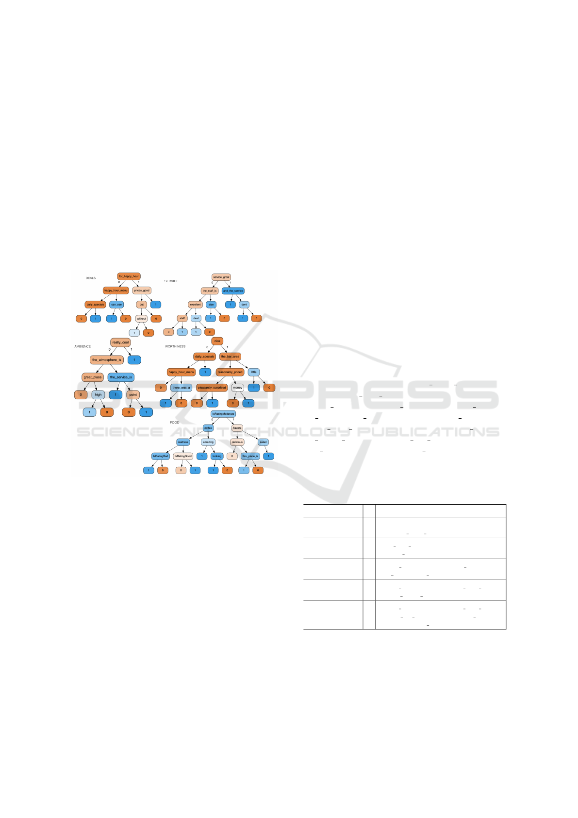
Example 1 (Running example: Classifying Yelp re-

views into 5 categories). The ”yelp reviews classiﬁca-

tion” is a categorization problem of reviews to know

whether a review positively comments on certain as-

pects such as food, service, ambiance, deals and wor-

thiness. The dataset contains more than 10000 re-

views from food and restaurant areas.

Input raw data is ﬁrst pre-processed and two types

of features are extracted that are i) textual features

consisting of unigrams, bigrams and trigrams and ii)

binary features representing rating 1-2 stars, 3 stars,

and 4-5 stars respectively. The classes are : F (Food),

S (Service), A (Ambience), D (Deals), W (Worthi-

ness). Assume now that we are considering the fol-

Figure 1: Binary Relevance based on decision trees on Yelp.

lowing review ”We went out with friends to have Mex-

ican food, the quesadillas was delicious and came

with a lot of cheese. We ﬁnd the place a little bor-

ing but the dining room seemed nice” accompanied

with a 4 stars rating. Assume also that we are given

the multi-label classiﬁer f depicted in Fig. 1 and con-

sisting in a Binary Relevance classiﬁer using decision

trees as base classiﬁers. The predicted outcome for

this review x is f (x)=(1, 0, 0, 0, 0).

3.2.1 Entire-Outcome Explanations

An entire-outcome explanation explains all the pre-

dicted labels simultaneously. Our feature-based ex-

planations are based on the deﬁnition of sufﬁcient

reason explanations and counterfactuals proposed ini-

tially for the multi-class case (Shih et al., 2018; Ig-

natiev et al., 2019a; Ignatiev et al., 2019b; Bouma-

zouza et al., 2021).

Entire-Outcome Sufﬁcient Reasons Explanations

An entire-outcome explanation (SR for short) iden-

tiﬁes the minimal part of a data sample x (namely,

the subset of features) capable to trigger the current

multi-label outcome. Formally,

Deﬁnition 2 (SR Explanations). Let x be a data in-

stance and y= f (x) be its prediction by the multi-label

classiﬁer f . An entire-outcome sufﬁcient reason ex-

planation

x is such that:

x ⊆ x (

x is a part of x),

2. ∀ ´x,

x ⊂ ´x : f ( ´x)= f (x) (

x sufﬁces to trigger f (x)),

3. There is no ˆx ⊂

x satisfying 1 and 2 (minimality).

While the two ﬁst conditions in Deﬁnition 2

search for parts of x allowing to ﬁre the same predic-

tion, the minimality one allows to ﬁnd parsimonious

explanations (in terms of the number of features in-

volved in the explanation).

Example 2 (Example 1 Continued). SR ex-

planations: In order to explain the prediction

y=(1, 0, 0, 0, 0) for the review in hand, an ex-

ample of sufﬁcient reason is [’IsRatingBad:0’,

’waitress:0’, ’looking:0’, ’this place is:0’, ’deli-

cious:1’, ’the staff is:0’, ’staff:0’, ’excellent:0’,

’service great:0’, ’great place:0’, ’really cool:0’,

’the atmosphere is:0’, ’daily specials:0’,

’happy hour menu:0’, ’prices good:0’,

’for happy hour:0’, ’the bar area:0’, ’pleas-

antly surprised:0’, ’reasonably priced:0’]. One can

check that this SR forces the ﬁve decisions trees to

predict y=(1, 0, 0, 0, 0) (see Table 2).

Table 2: An SR for the prediction y=(1, 0, 0, 0, 0).

Labels y Sufﬁcient Reason explanations

Food 1 [’IsRatingBad : 0’, ’waitress : 0’, ’looking

: 0’, ’this place is : 0’, ’delicious : 1’]

Service 0 [’the staff is : 0’, ’staff : 0’, ’excellent : 0’,

’service great : 0’]

Ambience 0 [’great place : 0’, ’really cool : 0’,

’the atmosphere is : 0’]

Deals 0 [’daily specials : 0’, ’happy hour menu :

0’, ’for happy hour : 0’]

Worthiness 0 [’daily specials : 0’, ’happy hour menu :

0’, ’the bar area : 0’, ’pleasantly surprised

: 0’, ’reasonably priced : 0’]

Entire-Outcome Counterfactual Explanations

Another important type of explanations that are ac-

tionable are the ones of counterfactuals. Given a tar-

get outcome ´y, an entire-outcome explanation (CF for

ICAART 2023 - 15th International Conference on Agents and Artiﬁcial Intelligence

344

short) is the minimal changes to be done in x in or-

der to obtain ´y. In other words, if for some reason,

one wants to force the classiﬁer to predict ´y, then a

counterfactual explanation is those minimal changes

´x needed to make on x such that f (x[ ´x])= ´y (the no-

tation x[ ´x] denotes the instance x where the variables

involved in ´x are inverted).

Deﬁnition 3 (CF Explanations). Let x be a complete

data instance and y= f (x) be its prediction by the

multi-label classiﬁer f . Given a target outcome ´y,

an entire-outcome counterfactual explanation

x of x

is such that:

x ⊆ x (

x is part of x),

2. f (x[

x]) = ´y (ﬁre target prediction),

3. There is no ˆx ⊂

x such that f (x[ˆx])= f (x[

x]) (minimal-

ity).

Example 3 (Example 2 Continued). Assume that

the initial prediction y is (1, 0, 0, 0, 0) and that the

target prediction ´y is (0, 1, 1, 1, 1). An example of

entire-outcome counterfactual is : [’delicious:1’,

’IsRatingModerate:0’ ’staff:0’, ’great place:0’,

’daily specials:0’, ’little:1’, ’the bar area:0’] . Table

3 shows how this CF forces each decision tree to

trigger the target outcome ´y.

Table 3: Example of entire-outcome CF explanation.

Labels y ´y Counterfactual explanations

Food 1 0 [’delicious : 1’, ’IsRatingModerate : 0’]

Service 0 1 [’staff : 0’]

Ambience 0 1 [’great place : 0’]

Deals 0 1 [’daily specials : 0’]

Worthiness 0 1 ’little : 1’, ’the bar area : 0’]

3.2.2 Fine-Grained Explanations

In practice, it can be more useful to get explanations

about a label or a subset of labels of interest rather

than an explanation for the entire prediction (a vec-

tor of k labels). We say that the Y

label is positively

predicted if Y

= 1, and negatively predicted if Y

= 0.

Fine-Grained Sufﬁcient Reasons Explanations

Similar to the deﬁnition of sufﬁcient reasons for the

entire-outcome, a ﬁne-grained sufﬁcient reason is

limited to explaining the part of y that is of interest

to the user.

Deﬁnition 4 (SR

Explanations). Let x be a data in-

stance, y= f (x) be its multi-label (entire) prediction by

the classiﬁer f and

y a subset of y representing the la-

bels of interest (

y can involve labels that are predicted

positively of negatively). A ﬁne-grained sufﬁcient rea-

son explanation

x of x is such that:

x ⊆ x (

x is a part of x),

2. ∀ ´x,

x ⊂ ´x : f ( ´x)=

y (

x sufﬁces to trigger

y),

3. There is no ˆx ⊂

x satisfying 1 and 2 (minimality).

Example 4 (Example 7 Continued). Assume we

want to explain the predictions regarding labels

”Food”, ”Service” and ”Ambience” (i.e (Y

1,Y

= 0,Y

= 0)). The following is an exam-

ple of a ﬁne-grained SR

explanation : [’IsRating-

Bad:0’, ’waitress:0’, ’looking:0’, ’this place is:0’,

’delicious:1’, ’the staff is:0’, ’staff:0’, ’excellent:0’,

’service great:0’, ’great place:0’, ’really cool:0’,

’the atmosphere is:0’].

Fine-Grained Counterfactual Explanations

Deﬁnition 5 (CF

Explanations). Let x be a data in-

stance, y= f (x) be its multi-label prediction by the

classiﬁer f . Let

y a subset of y representing the labels

of interest (namely, the labels to ﬂip). A ﬁne-grained

counterfactual explanation

x of x is such that:

x ⊆ x (

x is a part of x),

2. f (x[

x]) = y[

y] (inversion of labels into

y),

3. There is no ˆx ⊂

x such that, f (x[ ˆx])= f (x[

x]) (minimal-

ity)

The term y[

y] denotes the prediction y where labels

included in

y are inverted (set to the target outcome).

Example 5 (Example 4 Continued). Let us assume

that we want to invert the prediction of the labels

”Service” and ”Ambience” (i.e

y = (Y

= 1,Y

= 1)).

The following is an example of ﬁne-grained CF

ex-

planation: [ ’staff:0’, ’great place:0’].

3.3 Label-Based Explanations

Up to now, we explain the predictions of a classiﬁer

only using the features of the input data. Relying

solely on features to form symbolic explanations can

be problematic in terms of the clarity and relevance

of explanations to the user. As shown in the ﬁgures

of the example 6, explaining a complex concept or

label based solely on features can be difﬁcult for the

user to understand. In some cases, this aspect can be

greatly improved by exploiting relationships or struc-

tures between the labels. For instance, if a label Y

subsumed by a label Y

according to the multi-label

classiﬁer f , then clearly sufﬁcient reasons of Y

are

also sufﬁcient reasons for Y

. Other examples of re-

lations that can be easily extracted and exploited are

label equivalence and disjointedness.

The main advantage is that we will have a parsi-

monious explanation which will be easier for a user to

understand, and by reducing the number of the expla-

nations generated, it will simplify their presentation.

Symbolic Explanations for Multi-Label Classiﬁcation

345

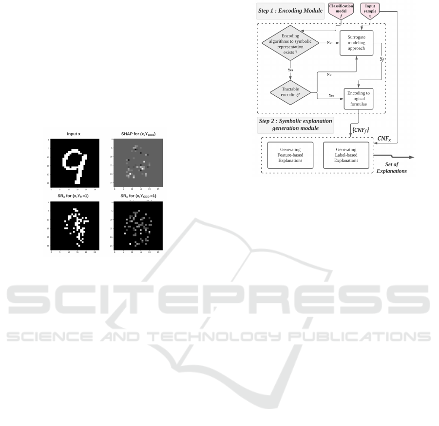
Example 6. Let us consider the example of dig-

its classiﬁcation using an augmented version of the

MNIST dataset with labels ”Odd”, ”Even” and

”Prime”. The existing labels Y

i∈0...9

indicate whether

the input image x is recognized as an i-digit while the

new labels Y

ODD

, Y

EV EN

and Y

PRIME

correspond re-

spectively to the labels ”Odd”, ”Even” and ”Prime”.

Assume an input image x, and its multi-label predic-

tion f (x)=(0, 0, 0, 0, 0, 0, 0, 0, 0, 1, 1, 0, 0) (namely, x is

predicted to be the digit ”9” and ”Odd”), we have the

following explanations:

Figure 2: Feature-based explanations for a sample from

augmented MNIST dataset.

4 A MODEL-AGNOSTIC

SAT-based APPROACH

As mentioned in the introduction, our approach

for providing symbolic explanations is agnostic and

declarative. It is based on modeling the multi-label

classiﬁer and our explanation enumeration problems

as variants of the propositional satisﬁability problem

(SAT) exactly in the spirit of ASTERYX (Bouma-

zouza et al., 2021). The modeling goes through two

steps: a ﬁrst step for encoding the multi-label classi-

ﬁer in an ”equivalent” (or ”faithful” in case of using

a surrogate model) canonical symbolic representation

then a second step for enumerating the explanations.

Before diving into more details, Fig. 3 depicts a gen-

eral overview of our approach:

4.1 Step 1: Classiﬁer Modeling

The aim of this step is to associate the multi-label

classiﬁer with a symbolic an equivalent/faithful sym-

bolic representation that can be processed by a SAT-

based oracle to enumerate our symbolic explanations.

As shown in Fig. 3, two cases are considered:

- Direct Encoding : Some machine learning mod-

els have direct encoding in conjunctive normal form

Figure 3: Overview of the proposed approach.

(CNF). For instance, the authors in (Narodytska et al.,

2018) proposed a CNF encoding for Binarized Neu-

ral Networks (BNNs) for veriﬁcation purposes. The

authors in (Shih et al., 2019) proposed algorithms for

compiling Naive and Latent-Tree Bayesian network

classiﬁers into decision graphs. Hence, in some cases,

a multi-label classiﬁer can be directly and equiva-

lently encoded in CNF. For instance, the Binary Rel-

evance classiﬁer using decision trees as base classi-

ﬁers can be equivalently encoded in CNF as illus-

trated in our running example (same thing holds of

random forests, Binarized Neural Networks and some

Bayesian network classiﬁers). The idea is to associate

a CNF Σ

with each base classiﬁer f

such that the

binary prediction of f

for a data instance x is cap-

tured by the truth value or consistency of Σ

and Σ

(Σ

stands for the CNF encoding of the data instance

x). Formally, f

is said to be equivalent to Σ

iff for

any data instance x :

∧ Σ



> if f

(x) = 1

⊥ otherwise.

(1)

Where > means that the conjunction of Σ

and Σ

is satisﬁable, corresponding to a positive prediction.

Similarly, ⊥ means that the conjunction of Σ

and Σ

is unsatisﬁable (in case of negative prediction).

- Surrogate Modeling : In case the multi-label clas-

siﬁer cannot be directly encoded in CNF or in case the

encoding is intractable, our approach proceeds by as-

sociating with the multi-label classiﬁer a faithful sur-

rogate model that can be encoded in CNF. In addi-

tion to allowing the handling of any multi-label clas-

siﬁer, the surrogate modeling offer another useful ad-

vantage that is providing local explanations. Indeed,

it is challenging to explain a model’s prediction over

the whole dataset where the decision boundary may

not be easily distinguished. The surrogate model built

ICAART 2023 - 15th International Conference on Agents and Artiﬁcial Intelligence

346

locally will make it possible to provide explanations

in the neighborhood of x. Our approach associates a

surrogate model s

for each label Y

. The surrogate

model s

is trained on the vicinity of the data sample

x using the original training instances with the pre-

dictions from the MLC model as targets or generated

data through perturbing the input instance x. A good

surrogate model is the one able to ensure a good trade-

off between a high faithfulness to the initial model and

tractability of the CNF encoding.

Example 7. Let us continue our running example.

The encoding of the decision trees of Fig. 1 into

CNF is direct as shown in the following (encoding

a decision tree in CNF comes down to encoding the

paths leading to leaves labeled 0).

Food y

⇔ (IsRatingModerate ∨ co f f ee ∨ waitress ∨

¬IsRatingBad) ∧

(IsRatingModerate ∨ co f f ee ∨ ¬waitress ∨

IsRatingGood) ∧

(IsRatingModerate ∨ ¬co f f ee ∨ ¬amazing¬looking) ∧

(¬IsRatingModerate ∨ f lavors ∨ delicious) ∧

(¬IsRatingModerate ∨ f lavors ∨ ¬delicious ∨

¬this place is)

Service y

⇔ (service great ∨ the sta f f is ∨ excellent ∨ sta f f )∧

(service great ∨ the sta f f is ∨ ¬excellent ∨ ¬deal) ∧

(service great ∨ ¬the sta f f is ∨ ¬size) ∧

(¬service great ∨ ¬and the service ∨ ¬dont)

Ambiencey

⇔ (really cool ∨ the atmosphere is ∨ great place)∧

(really cool ∨ the atmosphere is ∨ ¬great place ∨

¬high) ∧

(really cool ∨ ¬the atmosphere is ∨ ¬the service is ∨

point)

Deals y

⇔ ( f or happy hour ∨ happy hour menu ∨ daily specials)

∧

( f or happy hour ∨ ¬happy hour menu¬can see) ∧

(¬ f or happy hour ∨ prices good ∨ ¬out) ∧

(¬ f or happy hour ∨ prices good ∨ out ∨¬without)

Worth y

⇔ (nice ∨ daily specials ∨ happy hour menu) ∧

(nice ∨ daily specials ∨ ¬happy hour menu ∨

¬there was a) ∧

(¬nice ∨ the bar area ∨ reasonably priced ∨

pleasantly sur prised) ∧

(¬nice ∨the bar area ∨ ¬reasonably priced ∨money) ∧

(¬nice ∨ ¬the bar area ∨ ¬little)

Once the encoding step is achieved, we can rely on

SAT-based oracles to provide explanations as follows:

4.2 Step 2: Explanation Enumeration

Recall that in Step 2 we are given a set of CNFs

,..,Σ

encoding the MLC f and a data instance x

encoded in CNF and denoted Σ

. The aim is to ex-

plain the prediction y= f (x). Recall also that in order

to provide sufﬁcient reasons or counterfactuals for a

given label Y

, we rely on a SAT oracle on Σ

and Σ

In the following, let SR(x, s

) (resp. CR(x, s

)) denote

the set of sufﬁcient reasons (resp. counterfactuals) to

explain individual prediction s

(x). Such explanations

are obtained thanks to a SAT-based oracle (see for in-

stance (Boumazouza et al., 2021) how one can use a

SAT oracle to provide sufﬁcient reasons and counter-

factuals for binary classiﬁers).

4.2.1 Feature-Based Explanations

Depending on the type of explanations to provide, our

approach proceeds as follows:

- Entire-Outcome Sufﬁcient Reasons SR: Since we

can provide sufﬁcient reasons for each label Y

, then it

sufﬁces to combine (join) an SR from each classiﬁer

to form an SR for the whole outcome as shown in

the example of Table 2.

- Entire-Outcome Counterfactuals CF: Similar to

sufﬁcient reasons, one can form entire-outcome coun-

terfactual CF

as far as we have counterfactuals CF

for each label Y

. More precisely, let the MLC f pre-

dict y for x (namely, f (x)=y). Let us assume that

the user wants to force the prediction to y

. Then, an

entire-outcome CF is formed by joining a counterfac-

tual from each CF

(see example in Table 3).

- Fine-Grained Sufﬁcient Reasons SR

: For ﬁne-

grained explanations, we proceed in a similar way

while restricting to the part y

⊆y of interest to the user.

Namely, given sufﬁcient reasons for each label y

∈y

then joining an SR

from each classiﬁer f

with y

∈y

is enough to form an SR

for the partial outcome y

shown in Example 4.

- Fine-Grained Counterfactuals CF

: Given coun-

terfactuals for each label y

∈y

, then joining an CF

from each classiﬁer f

such that y

∈y

allows to build

an CF

allowing to obtain y

as in Example 5.

4.2.2 Label-Based Explanations

Recall that label-based explanations denote structural

relationships between labels. In order to extract some

relationships, one can also rely on a SAT-based ora-

cle since each individual labels Y

is associated with a

CNF Σ

. Hence, checking whether some relationships

hold between subsets of labels comes down to check-

ing the corresponding logical relationships between

CNF formulas.

For instance, assume we are given an input x and

the we want to check whether Y

≡Y

(label equiva-

lence relation) in the vicinity of x. We can easily

check if the CNF Σ

is logically equivalent to Σ

which case they must share the same models. Another

simple method consists simply in checking if for any

prediction y

= f (x

) such that x

is an instance from the

Symbolic Explanations for Multi-Label Classiﬁcation

347

Table 5: Evaluating the CNF encoding over different datasets.

Dataset radius avg RF’s

accuracy

min CNF

size

avg CNF size max CNF size min

enc runtime(s)

avg

enc runtime(s)

max

enc runtime(s)

YELP Review Analysis 60 92.67% 96/232 4827/13004 13732/36864 0.48 3.29 13.73

180 92.73% 4625/12416 6812/18395 15963/428941 2.97 4.64 15.32

Augmented MNIST 150 93.97% 509/1268 12095/32353 14308/38344 0.68 12.58 16.13

250 96.27 423/1119 9556/25455 15105/40530 1.35 7.93 14.41

IMDB Movie Genre Pred 30 99.53% 863/2344 1282/3533 3149/8558 0.82 1.09 2.73

Patient Characteristics

(NYS15)

63 96.73% 2446/6615 7887/21370 11305/30594 1.91 6.73 10.12

neighborhood of x that Y

=1 iff Y

=1.

5 EMPIRICAL EVALUATION

Due to the page limit, this study concerns only

feature-based explanations. The datasets used in our

experiments are publicly available and can be found

at Kaggle or at UCI. Numerical and categorical at-

tributes are binarized. The textual datasets used are

pre-preprocessed and binarized. In order to enu-

Table 4: Properties of the different data-sets used.

Dataset #instances #classes #features data type

Augmented MNIST 70000 13 784 Images

Yelp Review Analysis 10806 5 671 Textual

IMDB Movie Genre

Prediction

65500 24 30 Textual

Patient Characteristics

Survey (NYS 2015)

105099 5 63 Textual/

Numeric

merate our symbolic explanations for binary classi-

ﬁers, we rely on two SAT-based oracles: the enu-

meration of counterfactuals is done using the enumcs

tool(Gr

egoire et al., 2018) and the sufﬁcient rea-

sons are enumerated using the PySAT (Ignatiev et al.,

2018) tool. The time limit for the enumeration of

symbolic explanations was set to 300 seconds.

5.1 Results

In order to generate entire-outcome explanations,

each base classiﬁer of the a binary relevance (BR)

model is approximated using a random forest and then

encoded into a CNF. Table 5 lists the average size

and time of the encoding step computed over surro-

gate models. We can see that the average accuracy of

the surrogate random forest classiﬁers is high mean-

ing that the surrogate models can achieve high faith-

fulness levels wrt. the MLC. Regarding the size of

the generated CNFs expressed as the number of vari-

ables (#Vars) and number of clauses (#Clauses), one

can see that it is tractable and it is easily handled by

the SAT-solver (in Step 2).

Table 6 shows the results of enumerating both suf-

ﬁcient reasons and counterfactuals. Using local sur-

rogate models over multiple values of the radius, the

symbolic explanations of each base classiﬁer are enu-

merated, and then the average is computed and given

in Table 6 and Table 7. The average time necessary

to enumerate all the explanations for a given instance,

this latter varies between 2 and 20 seconds. The same

ﬁnding holds for the number of explanations where

one can see that on average this number increases pro-

portionally to the size of the feature set. We also no-

tice that the number of SR explanations is of the same

order as the number of CF ones. Interestingly enough,

one can notice that the time required to ﬁnd one sufﬁ-

cient reason (resp. counterfactual) explanation is very

negligible, meaning that the proposed approach is fea-

sible in practice.

6 CONCLUDING REMARKS

This paper proposed a declarative and model-agnostic

multi-label classiﬁcation explanation method. We de-

ﬁned several symbolic explanation types and showed

how we can enumerate them using the existing SAT-

based oracles. We introduced the concept of the label-

based explanations in order to take advantage of the

structural relationships between labels in order to re-

duce the number of generated explanations and im-

prove their presentation to the user. It is worth notic-

ing that the contributions of this work are not sim-

ple extensions from the multi-class framework to the

multi-label one since there are, for example, concepts

speciﬁc to the multi-label case such as label-based

and ﬁne-grained explanations.

ACKNOWLEDGMENT

This work was supported by the R

egion Hauts-de-

France.

ICAART 2023 - 15th International Conference on Agents and Artiﬁcial Intelligence

348

Table 6: Enumeration of entire-outcome counterfactual explanations.

Dataset radius min #CFs avg #CFs max #CFs enumtime One

CF (s)

min enumtime (s) avg enumtime (s) max enumtime (s)

YELP Review Analysis

60 1891 2025 6858 ≤ 10

−3

≤ 10

−3

2.29 13.46

180 2601 3203 9693 ≤ 10

−3

0.009 4.5 29.97

Augmented MNIST

150 96 4971 9347 ≤ 10

−3

0.02 15.61 33.27

250 1158 5027 11323 ≤ 10

−3

1.77 15.9 45.36

IMDB Movie Genre Pred 30 5 14 22 ≈ 0 0.13 2.78 7.47

Patient Characteristics (NYS15) 63 134 1052 2399 ≤ 10

−4

0.15 2.83 9.37

Table 7: Enumeration of entire-outcome sufﬁcient reasons explanations.

Dataset radius min #SRs avg #SRs max #SRs enumtime One

SR (s)

min enumtime (s) avg enumtime (s) max enumtime (s)

YELP Review Analysis 60 13116 23167 38620 0.028 10.94 19.37 31.95

Augmented MNIST 150 11292 11956 12621 0.053 12.26 13.06 13.85

IMDB Movie Genre Pred 30 3 41.83 161 0.004 0.003 0.02 0.07

REFERENCES

Boumazouza, R., Cheikh-Alili, F., Mazure, B., and Tabia,

K. (2021). Asteryx: A model-agnostic sat-based ap-

proach for symbolic and score-based explanations.

In Proceedings of the 30th ACM International Con-

ference on Information & Knowledge Management,

pages 120–129.

Chen, S. (2021). Interpretation of multi-label classiﬁcation

models using shapley values. CoRR, abs/2104.10505.

Ciravegna, G., Giannini, F., Gori, M., Maggini, M., and

Melacci, S. (2020). Human-driven fol explanations

of deep learning. In IJCAI, pages 2234–2240.

egoire,

E., Izza, Y., and Lagniez, J.-M. (2018). Boosting

mcses enumeration. In IJCAI, pages 1309–1315.

Ignatiev, A., Morgado, A., and Marques-Silva, J. (2018).

PySAT: A Python toolkit for prototyping with SAT or-

acles. In SAT, pages 428–437.

Ignatiev, A., Narodytska, N., and Marques-Silva, J. (2019a).

Abduction-based explanations for machine learning

models. In Proceedings of the AAAI Conference on

Artiﬁcial Intelligence, volume 33, pages 1511–1519.

Ignatiev, A., Narodytska, N., and Marques-Silva, J.

(2019b). On relating explanations and adversarial ex-

amples. In Advances in Neural Information Process-

ing Systems, volume 32.

Lundberg, S. M. and Lee, S.-I. (2017). A uniﬁed ap-

proach to interpreting model predictions. In Guyon,

I., Luxburg, U. V., Bengio, S., Wallach, H., Fer-

gus, R., Vishwanathan, S., and Garnett, R., editors,

Advances in Neural Information Processing Systems,

volume 30. Curran Associates, Inc.

Narodytska, N., Kasiviswanathan, S., Ryzhyk, L., Sagiv,

M., and Walsh, T. (2018). Verifying properties of

binarized deep neural networks. In Proceedings of

the AAAI Conference on Artiﬁcial Intelligence, vol-

ume 32.

Panigutti, C., Guidotti, R., Monreale, A., and Pedreschi, D.

(2019). Explaining multi-label black-box classiﬁers

for health applications. In International Workshop on

Health Intelligence, pages 97–110. Springer.

Reiter, R. (1987). A theory of diagnosis from ﬁrst princi-

ples. Artiﬁcial intelligence, 32(1):57–95.

Ribeiro, M. T., Singh, S., and Guestrin, C. (2016). ” why

should i trust you?” explaining the predictions of any

classiﬁer. In Proceedings of the 22nd ACM SIGKDD

2016, pages 1135–1144.

Ribeiro, M. T., Singh, S., and Guestrin, C. (2018). Anchors:

High-precision model-agnostic explanations. In Pro-

ceedings of the AAAI Conference on Artiﬁcial Intelli-

gence, volume 32.

Shih, A., Choi, A., and Darwiche, A. (2018). A sym-

bolic approach to explaining bayesian network clas-

siﬁers. In IJCAI-18, pages 5103–5111. International

Joint Conferences on Artiﬁcial Intelligence Organiza-

tion.

Shih, A., Choi, A., and Darwiche, A. (2019). Compiling

bayesian network classiﬁers into decision graphs. In

Proceedings of the AAAI-19, volume 33, pages 7966–

7974.

Singla, K. and Biswas, S. (2021). Machine learning explan-

ability method for the multi-label classiﬁcation model.

In 2021 IEEE 15th International Conference on Se-

mantic Computing (ICSC), pages 337–340. IEEE.

Symbolic Explanations for Multi-Label Classiﬁcation

349