Sequential Spatial Transformer Networks for Salient Object

Classiﬁcation

David Dembinsky

1,2,∗

, Fatemeh Azimi

1,2,∗

, Federico Raue

, J

orn Hees

, Sebastian Palacio

and Andreas Dengel

1,2

TU Kaiserslautern, Germany

German Research Center for Artiﬁcial Intelligence (DFKI), Germany

{ﬁrstname.lastname}@dfki.de

Keywords:

Sequential Spatial Transformer Networks, Reinforcement Learning, Object Classiﬁcation.

Abstract:

The standard classiﬁcation architectures are designed and trained for obtaining impressive performance on

dedicated image classiﬁcation datasets, which usually contain images with a single object located at the image

center. However, their accuracy drops when this assumption is violated, e.g., if the target object is cluttered

with background noise or if it is not centered. In this paper, we study salient object classiﬁcation: a more

realistic scenario where there are multiple object instances in the scene, and we are interested in classifying

the image based on the label corresponding to the most salient object. Inspired by previous works on Rein-

forcement Learning and Spatial Transformer Networks, we propose a model equipped with a trainable focus

mechanism, which improves classiﬁcation accuracy. Our experiments on the PASCAL VOC dataset show that

the method is capable of increasing the intersection-ver-union of the salient object, which improves the clas-

siﬁcation accuracy by 1.82 pp overall, and 3.63 pp for smaller objects. We provide an analysis of the failing

cases, discussing different aspects such as dataset bias and saliency deﬁnition on the classiﬁcation output.

1 INTRODUCTION

With the advancement of deep learning techniques

during the last decade (Krizhevsky et al., 2012;

Vaswani et al., 2017), these methods achieve impres-

sive performance in a variety of tasks such as image

classiﬁcation and object detection (He et al., 2015;

Ren et al., 2015). The majority of architectural ad-

vances based on Convolutional Networks (Xie et al.,

2017; Szegedy et al., 2017) or Transformer Networks

(Dosovitskiy et al., 2020) evaluate on high-quality

data such as CIFAR (Krizhevsky et al., 2009) or Ima-

genet (Deng et al., 2009). However, a side-product of

focusing on increasing the model accuracy on special-

ized and curated datasets is the lack of out-of-domain

generalization (Hendrycks and Dietterich, 2019) and

poor performance on images where the region of in-

terest (RoI) is not placed in the center of the image, let

alone if the scene is cluttered (Jaderberg et al., 2015;

Azimi et al., 2019).

In this paper, we study the task of salient object

classiﬁcation: A setup in which we aim at classifying

the most salient object in a scene where there are mul-

tiple object instances. Previous work has proposed

Equal contribution

various solutions for this task including attention by

(Mnih et al., 2014) or employing spatial transformer

networks (STN), transforming the input such that it is

easier to classify (Jaderberg et al., 2015; Azimi et al.,

2019); however, these methods were mainly applied

to simplistic scenarios and synthetic datasets.

In this work, we build on top of the Sequen-

tial Spatial Transformer Network (SSTN) algorithm

(Azimi et al., 2019). We extend their work by

multiple architectural and design improvements and

evaluate our model on the challenging real-world

dataset PASCAL VOC (Everingham et al., 2010). We

choose this method as the RL-based solution in (Az-

imi et al., 2019) allows us to employ a variety of non-

differentiable training objectives.

Our main hypothesis is that zooming in on the

salient object and cropping out secondary objects re-

garded as clutter is beneﬁcial for the classiﬁer. Hence,

increasing the Intersection over Union (IoU) of the

salient object (i.e. the ratio between the salient ob-

ject’s bounding-box area and the image area) can be

used as a training signal. We study this assumption in

Section 4.3.1.

Thanks to the availability of object detection

information in PASCAL VOC (Everingham et al.,

2010), we use bounding-box information to compute

328

Dembinsky, D., Azimi, F., Raue, F., Hees, J., Palacio, S. and Dengel, A.

Sequential Spatial Transformer Networks for Salient Object Classiﬁcation.

DOI: 10.5220/0011667100003411

In Proceedings of the 12th International Conference on Pattern Recognition Applications and Methods (ICPRAM 2023), pages 328-335

ISBN: 978-989-758-626-2; ISSN: 2184-4313

 2023 by SCITEPRESS – Science and Technology Publications, Lda. Under CC license (CC BY-NC-ND 4.0)

the IoU of different object instances in the scene. In-

stead of relying on human annotations for identifying

the salient object, we resort to the following approx-

imation: we assume object size as an estimator for

saliency and consider the largest object as the salient

one. We extend the algorithm proposed in (Azimi

et al., 2019) by employing Q-Learning, which is a

more effective algorithm in terms of scaling to high

dimensional input data such as images. Moreover, we

propose reward-shaping functions that attempt to di-

rectly increase the IoU of the salient object, result-

ing in improved classiﬁcation accuracy. Our method

named DQ-SSTN increases the IoU of the salient ob-

ject by 11.31 pp and the overall classiﬁcation accu-

racy by 1.82 pp. We observe that our method is espe-

cially effective for smaller objects (objects that cover

less than 20 percent of the image area), where we ob-

tain an improvement of 3.63 pp in accuracy. In Sec-

tion 4.4 we study the effect of the dataset characteris-

tics and saliency assumptions in failure scenarios.

2 RELATED WORK AND

BACKGROUND

In this section, we provide the preliminaries used

as the foundation of our work. We brieﬂy give an

overview of the utilized algorithms from the rein-

forcement learning literature, followed by an intro-

duction to Sequential Spatial Transformer Networks.

2.1 Reinforcement Learning

Reinforcement Learning (RL) is a learning paradigm

for training a learner (agent) by maximizing an ob-

jective via interacting with an environment and learn-

ing from the acquired experiences (Sutton and Barto,

2018). The RL framework is based on a Markov De-

cision Process (MDP) consisting of a set of states s,

actions a, and rewards r. The goal is to train an agent

which maximizes the reward function via searching

for the optimal action-selection policy through inter-

actions with the environment, as shown in Figure 1.

Each action selection results in receiving a reward and

a change in the current state.

The proposed algorithms for ﬁnding the optimal

action policy can be categorized into two main groups

of Policy Gradient and Q-learning. In this paper, we

utilize Q-learning due to its good performance in pro-

cessing high-dimensional states such as images (Mnih

et al., 2013). In Q-learning, the model learns a value

function q

∗

that estimates the expected reward for

each state-action pair. This function is learned based

on the Bellman Optimality equation:

Agent

Environment

Figure 1: The episodic MDP: First the agent observes the

environment’s state s and selects an action a which changes

the state to s

′

. Based on the impact of the action, the agent

receives the reward r. We train the agent to choose a se-

quence of actions leading to the maximum expected reward.

∗

(s, a) = r(s, a) + γmax

′

∗

′

(s, a), a

′

) (1)

where γ is a hyperparameter and θ represents the net-

work’s parameters. Since Equation 1 is greedy (max

operator) and initially the model is not trained, we use

the ε-greedy strategy, a trade-off between exploration

of the state-action space and exploitation of the ex-

pected rewards (Equation 2). Exploration decreases

with the number of taken steps n with decay d:

a =







rand

, if p < ε

end

+ (1 − ε

end

) · e

−

argmax

ˆa

∗

(s, ˆa), otherwise

(2)

rand

corresponds to an action selected randomly, p ∼

U(0, 1), and ε

end

and d are hyperparameters.

In Equation 1, there is a strong correlation be-

tween consecutive updates, which is detrimental to

the training procedure. This limitation is addressed

by utilizing a replay memory (Mnih et al., 2013), as a

way to break the correlation between the training sam-

ples. In the replay memory, each experience (s, a, r, s

′

)

is stored in a buffer and then drawn at random to per-

form a training step. Since the update rule in Equa-

tion 1 is dependent on the old parameters itself (θ), a

target network is additionally used for predicting the

expected reward (Mnih et al., 2015). The target net-

work has an identical architecture as the agent net-

work (q in Equation 1). It is not trained by gradient

descent, but its weights are periodically updated from

the agent network.

2.2 Spatial Transformer Networks

The Spatial Transformer Network (STN) (Jaderberg

et al., 2015) is a network architecture proposed to

learn modifying the input image by generating pa-

rameters of an afﬁne transformation. The network’s

parameters are trained by minimizing a differentiable

objective such as classiﬁcation loss. (Azimi et al.,

2019) propose a Sequential Spatial Transformer Net-

work (SSTN), which uses RL to ﬁnd the optimal

Sequential Spatial Transformer Networks for Salient Object Classiﬁcation

329

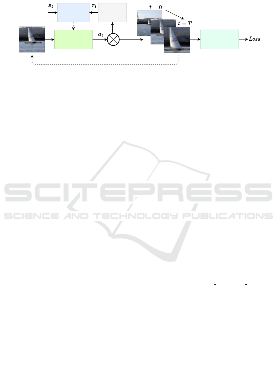
Q Network

(Agent)

Replay

Memory

Classifier

Reward

Function

Bilinear Sampler

Figure 2: The overall architecture of DQ-SSTN. Our model sequentially modiﬁes the input image by applying a series of

simple and discrete transformations (a

) selected by an agent trained to maximize the overall obtained reward (r

transformation. Rather than generating continuous

transformation parameters, they decompose the trans-

formation into a sequence of discrete and predeﬁned

simple transformations, which are chosen iteratively.

We extend their approach, as the RL-based formu-

lation allows us to work with non-differentiable ob-

jectives, as discussed in the following section.

3 METHOD

In this section, we study the problem of salient ob-

ject classiﬁcation where saliency is determined based

on an object’s bounding-box size, as discussed fur-

ther in Section 4.1.1 Opposite to standard image clas-

siﬁcation models working with curated images cen-

tered around a single salient object (Krizhevsky et al.,

2009; Deng et al., 2009), we focus on a more realistic

scenario where input images are cluttered with multi-

ple objects and the network has to classify the image

based on the most salient object. Since the original

SSTN method (Azimi et al., 2019) is limited to pro-

cessing small, gray-scale images, our goal is to extend

this algorithm for working with real-world data.

While SSTN uses Policy Gradient for training the

RL agent, we employ the Q-learning algorithm as it

works better for higher-dimensional data. Addition-

ally, we experiment with a variety of reward func-

tions, that based on different metrics, aim to boost

the performance of the downstream classiﬁer. Thanks

to the RL-based framework, our model is ﬂexible to

work with non-differentiable training objectives. Fig-

ure 2 visualizes the overall architecture of our model.

As mentioned in Section 2.1, to describe the MDP

framework, we have to deﬁne state space, action set,

and reward functions. For the state space s

, we con-

sider the transformed image at time t which has un-

dergone a sequence of transformations (the actions

selected by the agent). Our action set a

consists of

6 discrete afﬁne transformations with ﬁxed parame-

ters including translation in 4 directions, zooming and

identity. Identity allows early stopping while training

in batches and using a ﬁxed transformation length T .

Regarding the reward r

, we initially experiment

with the functions proposed by (Azimi et al., 2019)

referred to as Continuous loss-reward and Discrete

Acc-reward. Continuous loss-reward is the difference

between the classiﬁcation loss before and after apply-

ing the selected action (hence the reward is positive

when reducing the loss value). Discrete Acc-reward

rewards the agent with +1 if the classiﬁer’s prediction

changes from incorrect to correct or −1 vice-versa.

We further explore the possibility of improving

the classiﬁer accuracy by learning to increase the IoU

of the salient object. To this end, we positively reward

the agent when the selected action results in increas-

ing the area of the salient object. This way, the agent

is encouraged to zoom around the salient object. This

reward named Continuous IoU-reward is deﬁned as:

(c iou)

= IoU

− IoU

t−1

(3)

We also experiment with the discrete version of

the IoU and refer to it as Discrete IoU-reward:

(d iou)











+1, if IoU

> IoU

t−1

−1, if IoU

< IoU

t−1

0, else

(4)

The last reward for training the model is a

weighted combination of loss-reward and IoU-

reward, using hyperparameters α and β:

(combined)

= α · r

(c loss)

+ β · r

(d iou)

(5)

The objective for training the classiﬁer is the stan-

dard cross-entropy loss, and for the DQ-SSTN we use

Huber loss, a loss that serves as a compound of abso-

lute and squared loss (Huber, 1964).

4 EXPERIMENTS

In this section, we provide the implementation details,

as well as an analysis of the obtained results on the

PASCAL VOC dataset (Everingham et al., 2010). The

code is publicly available

https://git.opendfki.de/david.dembinsky/dq-sstn

ICPRAM 2023 - 12th International Conference on Pattern Recognition Applications and Methods

330

4.1 Implementation Details

4.1.1 Dataset

For evaluation, we use PASCAL VOC (Everingham

et al., 2010), a real-world dataset with pictures con-

taining multiple objects from 20 object classes. The

dataset provides the bounding box and the category

of each object. We combine the versions of 2007 and

2012 to get as many images as possible, resulting in a

training set of 8218 and a test set of 8333 frames.

For the classiﬁcation ground-truth label, we con-

sider the category of the object with the largest

area. Consequently, the Top-1 accuracy depends on

whether the prediction corresponds to the largest vis-

ible object. As additional metrics, we use the Top-2

and Any accuracies for evaluation (we only optimize

over Top-1 accuracy). The Top-2 accuracy addition-

ally allows the prediction to be the second largest ob-

ject, and the Any accuracy permits the prediction to

match any object present within an image.

We highlight that using the PASCAL VOC dataset

for single-class labeling results in a non-uniform class

distribution, where class person has more than 1700

images compared to other classes, which range from

below 200 to 600 images per class. We discuss a pos-

sible bias towards the dominant class in Section 4.4.1.

4.1.2 Training Setup

The backbone of the classiﬁer and the Q-network con-

sists of a ResNet18 (He et al., 2015) where the last

fully connected layer is modiﬁed to match the num-

ber of the object classes and the number of actions,

respectively. ResNet18 is an architecture quite suc-

cessful in image classiﬁcation tasks, and the library

PyTorch (Paszke et al., 2017) provides pre-trained

weights. We downscale the input images to 224 × 224

to match the ResNet18s implementation and perform

horizontal ﬂipping augmentations to increase the va-

riety in the dataset. We document the best set of hy-

perparameters found by experimentation. The replay

memory stores 1000 transitions. The ε-greedy strat-

egy Equation 2 uses d = 50000 and ε

end

= 0.05. For

Q-Learning (Equation 1) we use γ = 0.95 and update

our target-net after 100 agent updates. We train our

model with Adam (Kingma and Ba, 2015) optimizer

and a learning rate of 5 · 10

−6

for 50 epochs. The

trajectories are constructed with a length of T = 10

transformations. The DQ-SSTN’s transformations in-

clude translation by 4 pixels in each cardinal direction

and zooming-in by a factor of 0.8. The weight factors

in Equation 5 used are α = 1 and β = 0.8.

4.2 Main Results

Table 1 provides a comparison between the baseline

classiﬁer without DQ-SSTN and our proposed DQ-

SSTN method using different reward functions. As

can be seen from the results, the best accuracy was ob-

tained employing the discrete IoU reward, improving

Top-1 accuracy by 1.82 pp, Top-2 accuracy by 1.86

pp and Any accuracy by 1.23 pp, respectively.

In Figure 3, we provide an analysis of the IoU and

classiﬁcation accuracy using the best-found setup. We

visualize the IoU of the target class before and af-

ter applying the transformations selected by our DQ-

SSTN model. To better understand the impact of the

transformations on objects with different sizes, we di-

vide the test-set images into 5 bins, considering the

initial IoU. Applying the DQ-SSTN transformations

leads to an average increase of 11.31 pp in the tar-

get class IoU (the dotted line in this ﬁgure shows the

average IoU per bin). Additionally, we evaluate the

classiﬁcation accuracy for each bin before and after

applying transformations. We observe that our model

is more effective in improving the classiﬁcation accu-

racy of smaller objects, increasing it by 3.63 pp for

objects with an IoU less than 20%. Interestingly, the

IoU of the right-most bin decreases while the accu-

racy increases; this behavior will be observed in Sec-

tion 4.3.1 again and discussed in Section 4.4.2.

Visual examples of the transformations learned by

our model are illustrated in Figure 7.

Figure 3: IoU and classiﬁcation accuracy before and after

applying the DQ-SSTN transformations. The dataset is split

into ﬁve bins according to the initial IoU. Classiﬁcation ac-

curacy changes are noted under each column. DQ-SSTN

is especially useful for smaller objects (ﬁrst bin) where the

classiﬁcation accuracy is improved by 3.63 pp.

4.3 Ablation

4.3.1 Correlation of IoU and Accuracy

The main idea behind our DQ-SSTN is to zoom in on

the most salient object. The underlying assumption is

that classiﬁcation accuracy improves with increasing

the target object’s IoU. To conﬁrm this, we run an ex-

periment where we construct multiple datasets, each

Sequential Spatial Transformer Networks for Salient Object Classiﬁcation

331

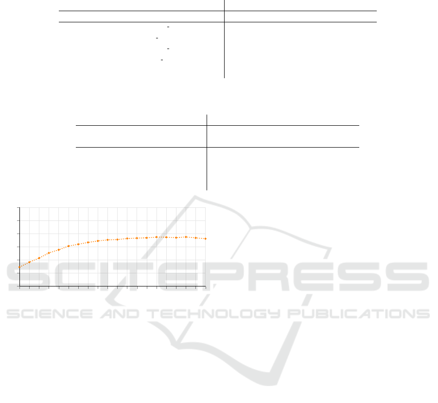
Table 1: Comparison of classiﬁcation accuracy of the baseline with our method when using different reward functions, on

PASCAL VOC (Everingham et al., 2010). We obtained the best results with the discrete IoU-based reward signal.

Method Top-1 (%) Top-2 (%) Any (%)

Baseline classiﬁer 80.04 82.97 88.22

Continuous loss-reward (r

c loss

) 80.84 83.75 88.83

Discrete Acc-reward (r

d acc

) 80.43 83.61 88.67

Continuous IoU-reward (r

c iou

) 80.15 83.09 88.19

Discrete IoU-reward (r

d iou

) 81.86 84.83 89.45

Weighted combination-reward (r

combined

) 81.54 84.56 89.27

Table 2: The impact of different hard-minig techniques tried on the classiﬁcation accuracy. Whilst the weight by accuracy

methods improved the Top-1 or Top-2 metric, respectively, by 0.06pp, we do not consider this as a noteworthy improvement.

Method Top-1 (%) Top-2 (%) Any (%)

Baseline classiﬁer 80.04 82.97 88.22

DQ-SSTN without hard mining 81.80 85.25 89.72

Weight reward by inverse IoU 81.40 85.13 89.60

Weight loss by inverse IoU 81.08 84.72 89.32

Weight reward by accuracy 81.86 84.83 89.45

Weight loss by accuracy 81.75 85.31 89.69

5 10 15 20 25 30 35 40 45 50 55 60 65 70 75 80 85 90 95 100

IoU of salient object in PASCAL VOC test-dataset

Classiﬁcation Accuracy

Manual IoU

Baseline

DQ-SSTN

Figure 4: Our experiment indicates a correlation between

salient object IoU and classiﬁcation accuracy (both in %).

Zooming on the target object (increase in IoU) leads to bet-

ter classiﬁcation accuracy for this object.

with a constant IoU enforced synthetically. To this

end, we determine the salient object by the size of the

bounding box and crop around it such that we achieve

a ﬁxed IoU for that object. Furthermore, we include

random translations to hinder the network from cheat-

ing and getting biased based on the positioning of the

object. This results in a dataset, where each image’s

salient object has the same, constant IoU.

After constructing 20 datasets with different IoUs,

we train and evaluate a classiﬁer on each dataset sep-

arately. As can be seen in Figure 4, an increase in the

IoU indeed leads to improved classiﬁcation accuracy.

We observe, that adjusting the IoU to more than 90%

reduces the accuracy. This shows that extreme zoom-

ing has a negative impact on performance, as infor-

mative parts of the object can be displaced out of the

classiﬁer’s focus (Selvaraju et al., 2016; Zhou et al.,

2016). We discuss this more in-depth in Section 4.4.2.

4.3.2 Hard Mining

Our PASCAL VOC dataset suffers from a consider-

able imbalance in both class distribution and IoU dis-

tribution. This imbalance might hurt performance as

the learned solution could be biased towards the dom-

inant category. Hard mining is a training technique

that has been proven effective (Shrivastava et al.,

2016; Dong et al., 2017) to alleviate the effect of data

imbalance by assigning a higher weight to underrep-

resented (therefore more challenging) data samples.

To this end, we experiment with multiple hard-

mining strategies and provide the results in Table 2.

As our overall objective consists of the classiﬁcation

and the reward maximization terms, we can perform

hard mining by re-weighting the classiﬁer’s loss or the

reward of the more challenging data samples.

Initially, we consider IoU as a measure of a

data sample hardness. Therefore, we reweigh ei-

ther the loss function or the reward signal by the in-

verse of IoU, assigning higher importance to sam-

ples with smaller IoU (Weight reward by inverse IoU

and Weight loss by inverse IoU). Surprisingly, our re-

sults did not improve with this technique. Next, we

reweigh the data samples based on the performance

of the baseline classiﬁer. If an image is classiﬁed

incorrectly, we assign a weight of 1 and, if it’s pre-

dicted correctly, a constant weight < 1. This assigns

higher importance to those images which are more

difﬁcult for our classiﬁer (Weight reward by accuracy

and Weight loss by accuracy). The results show small

improvements of 0.06 pp for either Top-1 or Top-2 ac-

curacy, hence, we do not ﬁnd these techniques useful

to our algorithm.

ICPRAM 2023 - 12th International Conference on Pattern Recognition Applications and Methods

332

4.4 Limitations

In this section, we provide a detailed analysis of the

results to better understand the impact of the dataset

and the assumptions that we made about object size

and saliency. We observe that the dominance of class

person biases the classiﬁer’s prediction. Additionally,

we show that deﬁning saliency is a non-trivial task

and can have a serious impact on the model.

4.4.1 Bias of the Person Class

One property of the PASCAL VOC dataset is an im-

balance in the class distribution. Based on object size,

about 20% of all images are assigned to person class.

As a result, we observe that the attention of our

DQ-SSTN gets drawn towards persons: If a person is

present in the scene, the classiﬁer is biased towards

classifying the image as person category. In Table 3,

we provide statistics for misclassiﬁcations consider-

ing whether a person is present as a secondary ob-

ject. It is clearly visible, that in cases where a person

is present, the classiﬁer is biased toward this class.

However, if there is none the image, the classiﬁer

does not overly tend towards predicting one. Note that

a random classiﬁer would select person class around

20% of the time, following the dataset distribution in

the training set.

This problem is introduced by the PASCAL VOC

dataset, as there are far more person objects through-

out the dataset than others.

Table 3: The prediction of the classiﬁer on images that were

predicted incorrectly. If there is a person present, the DQ-

SSTN has a high chance of focusing on it.

(%) pred. person pred. other

person present 39.37 60.63

person not present 11.15 88.85

4.4.2 Issues with Saliency Assumption

The way we changed the detection dataset into one

for classiﬁcation depends on our saliency assump-

tion: We assume the object with the biggest bounding

box to be the most salient one, as described in Sec-

tion 4.1.1. In this section, we investigate how often

and to which extent this assumption is violated and

how this impacts the performance of the DQ-SSTN.

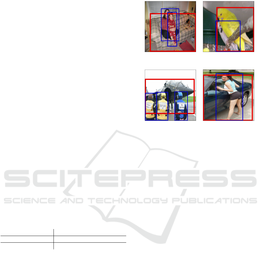
An example in contrast with our saliency assump-

tion is when a smaller object is located in front of a

bigger one. Consider a person sitting on a sofa (as

in Figure 5); in this scenario, humans consider the

person as the salient object, while based on our as-

sumption, the sofa is labeled as the salient category.

Interestingly, we observed that in most cases the clas-

30.88%

sofa

43.80%

bird

44.58%

aeroplane

54.27%

car

Figure 5: Visual examples where the main object intersects

with other objects. Red frames surround the largest ob-

ject, and blue frames the secondary ones. The value below

each image is the percentage of the largest (salient) object’s

bounding box that intersects with other bounding boxes and

the assigned true label is also given. The ﬁrst image is an

image below threshold th = 0.4 but still considered clut-

tered, and the second one is vice versa. The other two ex-

amples further highlight our choice of threshold.

siﬁer also predicts the front object as the correct class

(person in this example), but this is considered a mis-

classiﬁcation based on our evaluation.

To better understand this issue, we visualize the

overlap characteristics of our data in Figure 6. In this

ﬁgure, we see the portion of images in which the main

object (largest/salient) is not overlapping with other

objects in the scene, as well as the number of im-

ages in which the main object intersects with other

object instances considering different overlap thresh-

olds. For example, the column with th = 0.5 shows

the number of images in which the overlap between

the main and the secondary objects is lower or higher

than 50% of the main object area.

We observed that 41.35% of the images only have

one object and 10.76% of all images are accompanied

by secondary objects, but their bounding boxes do not

intersect with each other. This means that in 52.12%

of the images, our assumption about saliency strictly

holds. However, in 47.88% of the images, the salient

object is to some extent intersecting with (and pos-

sibly being occluded by) another object. Looking at

some qualitative examples (Figure 5), we consider a

threshold of th = 0.4 as critical; i.e. all images that

have more than 40% of their bounding-box concealed

Sequential Spatial Transformer Networks for Salient Object Classiﬁcation

333

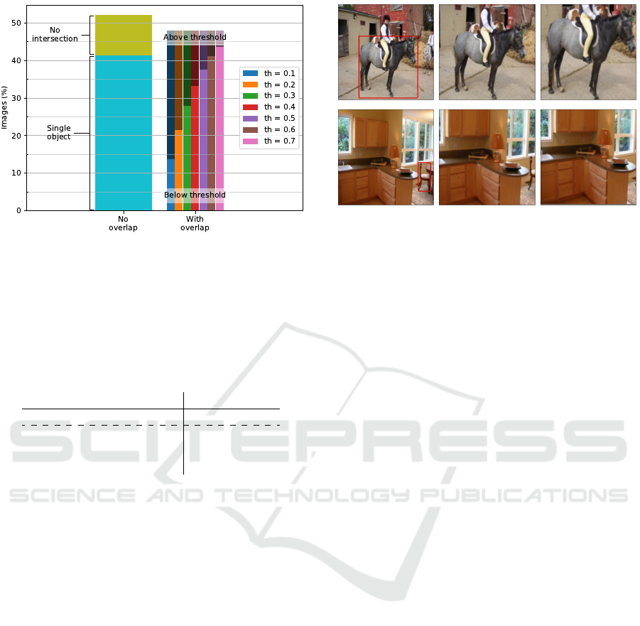
Figure 6: This histogram shows the composition of our

dataset regarding the relation between the most salient ob-

ject and overlapping objects. Depending on the selected

threshold, between 5%(th = 0.7) to 35%(th = 0.1) of all

images are to some extent covered by another object in-

stance, thus violating our assumption of saliency.

Table 4: DQ-SSTN classiﬁcation accuracy on each subset

of PASCAL VOC when categorized based on the overlap

threshold of 0.4 (as shown in Figure 6).

Accuracy (%)

Total 81.86

No clutter 86.05

Cluttered, below th = 0.4 82.83

Cluttered, above th = 0.4 64.88

by another object do not follow our saliency assump-

tion based on object size. Based on this threshold,

about 15% of the dataset conﬂict with our saliency

assumption.

To investigate the impact of our saliency assump-

tion on the DQ-SSTN performance, we divide the

dataset into three categories; the images with the main

object not covered by any other objects and the im-

ages in which the main object is covered by other in-

stances more or less than 40% (th = 0.4 in Figure 6)

We evaluate our model separately on each group and

present the results in Table 4. As expected, we ob-

serve that the classiﬁcation accuracy is signiﬁcantly

lower for the data in which the salient object has an

overlap of over 40% with other objects in the scene.

5 CONCLUSION AND FUTURE

WORK

In this paper, we study the task of salient object clas-

siﬁcation. We introduce DQ-SSTN, a Sequential Spa-

tial Transformer Network based on Deep Q-Learning.

Our model learns to zoom on the salient object by it-

t = 0 (Start) t = 5 t = 10 (End)

Figure 7: Visual examples of our DQ-SSTN model grad-

ually focusing on the salient object. The bounding box of

the largest object is visualized in red in the starting frame

(t=0). The ﬁrst row is an example of the DQ-SSTN work-

ing as expected. The second row is a failing case, where the

DQ-SSTN cannot ﬁnd the salient object and blindly zooms

in.

eratively selecting an afﬁne transformation to increase

the IoU of the largest object in an image. We experi-

mentally demonstrate the effectiveness of our method

in improving the classiﬁcation accuracy, especially

for smaller objects where we achieve an improvement

of 3.63 pp. Furthermore, we provide several abla-

tion studies to investigate the reason behind failure

scenarios. In future work, we plan to explore more

ﬂexible solutions by considering all objects within an

image during training favoring a multi-labeling ap-

proach where the DQ-SSTN successively classiﬁes

every object within the image. Moreover, we believe

working towards preparing a more dedicated dataset

free from class bias would beneﬁt our work.

ACKNOWLEDGMENT

This work was supported by the TU Kaiserslautern

CS PhD scholarship program, the BMBF project

ExplAINN (01IS19074), and the NVIDIA AI Lab

(NVAIL) program.

REFERENCES

Azimi, F., Raue, F., Hees, J., and Dengel, A. (2019). A

reinforcement learning approach for sequential spa-

tial transformer networks. In Tetko, I. V., K

urkov

V., Karpov, P., and Theis, F., editors, Artiﬁcial Neural

Networks and Machine Learning – ICANN 2019: The-

oretical Neural Computation, pages 585–597, Cham.

Springer International Publishing.

ICPRAM 2023 - 12th International Conference on Pattern Recognition Applications and Methods

334

Deng, J., Dong, W., Socher, R., Li, L.-J., Li, K., and Fei-

Fei, L. (2009). Imagenet: A large-scale hierarchical

image database. In 2009 IEEE conference on com-

puter vision and pattern recognition, pages 248–255.

Ieee.

Dong, Q., Gong, S., and Zhu, X. (2017). Class rectiﬁca-

tion hard mining for imbalanced deep learning. In

Proceedings of the IEEE International Conference on

Computer Vision, pages 1851–1860.

Dosovitskiy, A., Beyer, L., Kolesnikov, A., Weissenborn,

D., Zhai, X., Unterthiner, T., Dehghani, M., Min-

derer, M., Heigold, G., Gelly, S., Uszkoreit, J., and

Houlsby, N. (2020). An image is worth 16x16 words:

Transformers for image recognition at scale. CoRR,

abs/2010.11929.

Everingham, M., Van Gool, L., Williams, C. K., Winn, J.,

and Zisserman, A. (2010). The pascal visual object

classes (voc) challenge. International journal of com-

puter vision, 88(2):303–338.

He, K., Zhang, X., Ren, S., and Sun, J. (2015). Deep

residual learning for image recognition. CoRR,

abs/1512.03385.

Hendrycks, D. and Dietterich, T. (2019). Benchmarking

neural network robustness to common corruptions and

perturbations. In International Conference on Learn-

ing Representations.

Huber, P. J. (1964). Robust Estimation of a Location Param-

eter. The Annals of Mathematical Statistics, 35(1):73

– 101.

Jaderberg, M., Simonyan, K., Zisserman, A., and

Kavukcuoglu, K. (2015). Spatial transformer net-

works. In Cortes, C., Lawrence, N., Lee, D.,

Sugiyama, M., and Garnett, R., editors, Advances in

Neural Information Processing Systems, volume 28.

Curran Associates, Inc.

Kingma, D. P. and Ba, J. (2015). Adam: A method for

stochastic optimization. In Bengio, Y. and LeCun,

Y., editors, 3rd International Conference on Learn-

ing Representations, ICLR 2015, San Diego, CA, USA,

May 7-9, 2015, Conference Track Proceedings.

Krizhevsky, A., Hinton, G., et al. (2009). Learning multiple

layers of features from tiny images.

Krizhevsky, A., Sutskever, I., and Hinton, G. E. (2012). Im-

agenet classiﬁcation with deep convolutional neural

networks. In Pereira, F., Burges, C. J. C., Bottou, L.,

and Weinberger, K. Q., editors, Advances in Neural

Information Processing Systems, volume 25. Curran

Associates, Inc.

Mnih, V., Heess, N., Graves, A., et al. (2014). Recurrent

models of visual attention. Advances in neural infor-

mation processing systems, 27.

Mnih, V., Kavukcuoglu, K., Silver, D., Graves, A.,

Antonoglou, I., Wierstra, D., and Riedmiller, M. A.

(2013). Playing atari with deep reinforcement learn-

ing. CoRR, abs/1312.5602.

Mnih, V., Kavukcuoglu, K., Silver, D., Rusu, A. A., Ve-

ness, J., Bellemare, M. G., Graves, A., Riedmiller, M.,

Fidjeland, A. K., Ostrovski, G., et al. (2015). Human-

level control through deep reinforcement learning. na-

ture, 518(7540):529–533.

Paszke, A., Gross, S., Chintala, S., Chanan, G., Yang, E.,

DeVito, Z., Lin, Z., Desmaison, A., Antiga, L., and

Lerer, A. (2017). Automatic differentiation in pytorch.

In NIPS-W.

Ren, S., He, K., Girshick, R., and Sun, J. (2015). Faster

r-cnn: Towards real-time object detection with region

proposal networks. Advances in neural information

processing systems, 28.

Selvaraju, R. R., Das, A., Vedantam, R., Cogswell, M.,

Parikh, D., and Batra, D. (2016). Grad-cam: Why

did you say that? arXiv preprint arXiv:1611.07450.

Shrivastava, A., Gupta, A., and Girshick, R. (2016). Train-

ing region-based object detectors with online hard ex-

ample mining. In Proceedings of the IEEE conference

on computer vision and pattern recognition, pages

761–769.

Sutton, R. S. and Barto, A. G. (2018). Reinforcement learn-

ing: An introduction. MIT press.

Szegedy, C., Ioffe, S., Vanhoucke, V., and Alemi, A. A.

(2017). Inception-v4, inception-resnet and the impact

of residual connections on learning. In Thirty-ﬁrst

AAAI conference on artiﬁcial intelligence.

Vaswani, A., Shazeer, N., Parmar, N., Uszkoreit, J., Jones,

L., Gomez, A. N., Kaiser, Ł., and Polosukhin, I.

(2017). Attention is all you need. Advances in neural

information processing systems, 30.

Xie, S., Girshick, R., Doll

ar, P., Tu, Z., and He, K. (2017).

Aggregated residual transformations for deep neural

networks. In Proceedings of the IEEE conference on

computer vision and pattern recognition, pages 1492–

1500.

Zhou, B., Khosla, A., Lapedriza, A., Oliva, A., and Tor-

ralba, A. (2016). Learning deep features for discrim-

inative localization. In Proceedings of the IEEE con-

ference on computer vision and pattern recognition,

pages 2921–2929.

Sequential Spatial Transformer Networks for Salient Object Classiﬁcation

335