Clustering LiDAR Data with K-means and DBSCAN
Mafalda In
ˆ
es Oliveira
a
and Andr
´
e R. S. Marcal
b
Faculdade de Ci
ˆ
encias, Departamento de Matem
´
atica, Universidade do Porto,
Rua do Campo Alegre s/n 4169-007, Porto, Portugal
Keywords:
LiDAR Data, Clustering, DBSCAN, K-means, Validation.
Abstract:
Multi-object detection is an essential aspect of autonomous driving systems to guarantee the safety of self-
driving vehicles. In this paper, two clustering methods, DBSCAN and K-means, are used to segment LiDAR
data and recognize the objects detected by the sensors. The Honda 3D LiDAR Dataset (H3D) and BOSCH
data acquired within the THEIA project were the datasets used. The clustering methods were evaluated in
several traffic scenarios, with different characteristics, extracted from both datasets. To validate the clustering
results, five internal indexes were computed for each scenario tested. The available ground truth data for the
H3D dataset also enabled the computation of 3 basic external indexes and a composite external index, which is
newly proposed. A method to compute reference bounding boxes is presented using the available labels from
H3D. The overall results indicate that K-means outperformed DBSCAN in the internal validation indexes
Silhouette, C-index, and Calinski-Harabasz, and DBSCAN performed better than K-means in the Dunn and
Davies-Bouldin indexes. The external validation indexes indicated that DBSCAN produces the best results,
supporting the fact that density clustering is well-suited for LiDAR segmentation.
1 INTRODUCTION
There is great interest and effort in developing sys-
tems for self-driving vehicles. A major aspect of
these systems is the need to assure fully safe au-
tonomous driving. The vehicle’s sensors must thus
detect and identify all surrounding objects correctly.
Clustering methods can recognize patterns and con-
sequently extract relevant information from several
types of datasets. The topic of autonomous driving
can also benefit from these techniques since it is pos-
sible to detect 3D multi-objects from LiDAR obser-
vations. This paper addresses this topic, by perform-
ing an evaluation of two clustering methods: K-means
and DBSCAN. An experiment was carried out with
LiDAR data from two distinct datasets. A total of 9
validation indexes were used to evaluate the results
produced from both clustering methods - 5 internal
indexes, and 4 external indexes.
2 CLUSTERING METHODS
Clustering is an unsupervised machine-learning tech-
nique that allows one to find patterns and iden-
a
https://orcid.org/0000-0001-6871-6281
b
https://orcid.org/0000-0002-8501-0974
tify groups of similar observations in multivariate
data to extract relevant information. Thus, clus-
tering can be very helpful for forming groups ac-
cording to the objects observed by LiDAR. Different
datasets require different clustering methods chosen
from different categories of clustering (e.g. Partition-
ing Methods, Hierarchical Clustering, and Density-
based Clustering) (Xu and Tian, 2015). Within
these categories, K-means, DBSCAN, BIRCH, and
Expectation-Maximization Clustering using Gaussian
Mixture Models are the more commonly used cluster-
ing algorithms (Xu and Tian, 2015). DBSCAN might
be the most suitable clustering method for data with
arbitrary cluster shapes, which is the case of the data
collected from LiDAR sensors (Wang et al., 2019). In
this paper, a distance-based method (K-means) and a
density-based method (DBSCAN) were used.
2.1 K-means Clustering
K-means is a clustering method that looks for the divi-
sion of the data into K clusters and assigns each obser-
vation to the cluster that minimizes the within-cluster
sum of squares (Syakur et al., 2018). The objective is
to minimize S in equation (1), where X
i
and X
k
are the
i
th
and k
th
data points:
822
Oliveira, M. and Marcal, A.
Clustering LiDAR Data with K-means and DBSCAN.
DOI: 10.5220/0011667000003411
In Proceedings of the 12th International Conference on Pattern Recognition Applications and Methods (ICPRAM 2023), pages 822-831
ISBN: 978-989-758-626-2; ISSN: 2184-4313
Copyright
c
 2023 by SCITEPRESS – Science and Technology Publications, Lda. Under CC license (CC BY-NC-ND 4.0)

S =
K
∑
k=1
∑
C(i)=k
||X
i
− X
k
||
2
(1)
One of the disadvantages of this method is having
to choose an adequate value for K. In order to com-
pare the performance of K-means with DBSCAN, the
K-means method was applied with K equal to the
number of clusters returned by DBSCAN. In order to
ensure the ideal value for K, K-means was also tested
for all values between 2 and the value returned by DB-
SCAN. Additionally, it is necessary to notice that the
final result of the clustering depends on the initial lo-
cation of the cluster centers. Thus, to assure repro-
ducibility, the method was applied with fixed cluster
center locations.
2.2 DBSCAN Clustering
Density-Based Spatial Clustering of Applications
with Noise (DBSCAN) (Ester et al., 1996) is a data
clustering algorithm that given a set of points in some
space, groups together points based on a specified dis-
tance (e.g. Euclidean), that are close to each other. A
cluster only forms when a minimum number of points
(m), specified by the user, is assigned. In low-density
regions, some data points do not have a neighborhood
large enough to create a new cluster, so the algorithm
marks them as outliers. This method is helpful when-
ever the dataset has arbitrary shapes and densities, so
it can be useful for segmenting LiDAR data. The al-
gorithm has two parameters: the minimum number
of points that a cluster needs to be created (m) and a
fixed radius for the search of neighbors (ε).
A suitable choice for the parameter m is 2 times
the dimension of the data (Sander et al., 1998). For
the estimation of the ε value, a k-distance graph for
the data is designed where k is the parameter m (Ester
et al., 1996). The goal is to compute the distance from
each point in the data to its m-th nearest point and
then plot the sorted points in ascending order of their
m-distance value against those distances. The ideal
value for ε will be the point of maximum curvature.
The process is illustrated for a test scenario in section
5.1 (Figure 4).
3 CLUSTERING VALIDATION
Clustering validation is an essential step to evaluate
the clustering results. There are 3 types of clustering
validation procedures: external clustering validation,
internal clustering validation, and relative cluster val-
idation (Halkidi et al., 2001). Internal clustering vali-
dation is based on information intrinsic to the data and
uses the internal information of the clustering process
to evaluate the procedure. On the other hand, exter-
nal validation indexes compare the results of a cluster-
ing procedure to a pre-existing clustering structure - a
reference or ground truth data. Therefore, internal in-
dexes only use information about the dataset and clus-
tering results, whereas external indexes also require
independent data labels. Relative cluster validation
evaluates the clustering process by varying different
parameter values for the clustering method in analy-
sis.
Besides these 3 types of clustering validation pro-
cedures, the within-cluster variance can also be an
informative measure of the clustering results. The
Within Cluster Variance (V
WC
) indicates an estima-
tion of the dispersion of the observations within a
cluster and is computed using equation (2), where C
k
is the k cluster and x
k
is the mean feature vector for
cluster k.
V
WC
=
∑
x
i
∈C
k
||x
i
− x
k
||
2
(2)
This value should be interpreted carefully because
clusters with very few points will have low V
WC
val-
ues, which could not always imply that the clusters
have a low dispersion of their points.
In order to guarantee the safety of autonomous ve-
hicles, it is necessary to recognize the distance be-
tween the vehicle and the surrounding objects. There-
fore, the distance from the LiDAR to the clusters can
represent relevant information since the value indi-
cates how close an obstacle is from the car with the
LiDAR sensor, and collisions with obstacles can be
avoided. The Distance to LiDAR is calculated based
on the minimum point distance. The minimum dis-
tance between cluster A and a point X=(x,y,z) cor-
responding to the LiDAR sensor coordinates is com-
puted using equation (3), where d
e
is the Euclidean
distance.
D
SL
= min{d
e
(X, a) : a ∈ A} (3)
3.1 Internal Validation Indexes
3.1.1 Silhouette Index
The silhouette index (I
S
) measures the similarity of a
data point to its cluster compared to the similarity to
other clusters. The index is computed for every point
in the data using equation (4), where a(i) is the aver-
age dissimilarity of the i
th
object to all other objects in
the same cluster, and b(i) is the average dissimilarity
of the i
th
object with all objects in the closest cluster
(Arbelaitz et al., 2013).
I
S
(i) =
b(i) − a(i)
max{a(i), b(i)}
(4)
Clustering LiDAR Data with K-means and DBSCAN
823

The silhouette index ranges from −1 to 1, where
a value close to 1 suggests that the point is well-
matched to its cluster. A value of 0 means that the
point is on or very close to the decision boundary be-
tween two neighboring clusters. A negative value in-
dicates that the point could have potentially been as-
signed to the wrong cluster. To evaluate the results
overall, the mean of the index for the totality of points
is calculated.
3.1.2 Dunn Index
The Dunn Index (I
D
) intends to identify clusters with
a small variance between the points within the cluster
and, at the same time, guarantee that the distance be-
tween the group means is large. I
D
is computed using
equation (5), with δ(C
k
,C
l
) the intercluster distance
and ∆(C
k
) the intracluster distance, considering C
k
as
the k cluster and C
l
as the l cluster (Arbelaitz et al.,
2013);(Ramos, 2022).
I
D
(C) = min
C
k
∈C

min
C
l
∈C\C
k

δ(C
k
,C
l
)
max
C
k
∈C
{∆(C
k
)}

(5)
The Dunn Index ranges between 0 and ∞ and should
be maximized. A high value for I
D
means that the
observations in each cluster are close together and the
clusters are well separated.
3.1.3 Davies-Bouldin Index
The Davies-Bouldin Index (I
DB
) is defined as a ratio
between the within-cluster distances and the between-
cluster distances and is calculated using equation (6),
with S(C
k
) =
1
|C
k
|
∑
X
i
∈C
k
d
e
(X
i
,C
k
), k the total number
of clusters and d
e
the Euclidean distance (Arbelaitz
et al., 2013).
I
DB
(C) =
1
K
∑
C
k
∈C
max
C
l
∈C\C
k

S(C
k
) + S(C
l
)
d
e
(C
k
,C
l
)

(6)
The index should be minimized so it can be as close
to 0 as possible since the index is non-negative. A
value of 0 means that the average similarity is mini-
mum therefore the clusters are better defined.
3.1.4 DBCV Index
Density-Based Clustering Validation (I
DBCV
) is a val-
idation index for density-based clustering that can
be very helpful in evaluating clusters with arbitrary
shapes. The index is formulated based on a ker-
nel density function. The kernel function computes
the density of the objects and evaluates the within-
cluster and between-cluster density connectedness of
the clustering results. The exact formulation of the
DBCV index is more complex than the previous in-
dexes and can be seen in detail in (Moulavi et al.,
2014).
3.1.5 C-Index
The C-index (I
C
) compares the dispersion of data
clusters relative to the total dispersion in the dataset.
I
C
is computed using equation (7) and should be min-
imized until the ideal value 0 (Arbelaitz et al., 2013).
I
C
(C) =
S
w
(C) − S
min
(C)
S
max
(C) − S
min
(C)
(7)
where
S(C) =
∑
c
k
∈C
∑
x
i
,x
j
∈c
k
d
e
(x
i
, x
j
)
S
min
(C) =
∑
min(n
w
)
x
i
,x
j
∈X
d
e
(x
i
, x
j
)
S
max
(C) =
∑
max(n
w
)
x
i
,x
j
∈X
d
e
(x
i
, x
j
)
with X the entire dataset, x
i
, x
j
the data points and
d
e
the Euclidean distance.
3.1.6 Calinski–Harabasz Index
The Calinski-Harabasz index (I
CH
) compares the vari-
ance between clusters to the variance within each
cluster. A higher value for I
CH
indicates a better sep-
aration of the clusters. The index is calculated using
equation (8), where N is the total number of points
and the other symbols as defined for the indexes pre-
sented previously (Arbelaitz et al., 2013).
I
CH
(C) =
N − K
K − 1
∑
C
k
∈C
|C
k
|d
e
(C
k
, X)
∑
C
k
∈C
∑
X
i
∈C
k
d
e
(X
i
,C
k
)
(8)
The Calinski–Harabasz index is unbounded and it
should be maximized.
3.2 External Validation Indexes
To validate the clusters created from both algorithms,
3 basic external validation indexes were used: the
cluster index, the box index, and the label index. Con-
sidering that these 3 indexes emphasize different and
somehow complementary aspects, a composite index
is proposed - CEVI (Composite External Validation
Index).
3.2.1 Basic External Validation Indexes
The cluster index (IE
C
) compares the number of
points in a cluster that is inside the bounding box of
ICPRAM 2023 - 12th International Conference on Pattern Recognition Applications and Methods
824

the corresponding object (#C
BBx
) with the total num-
ber of points in that cluster (#C). IE
C
is calculated for
every cluster C using equation (9). The index intends
to identify the clusters that group together only one
object, meaning that a IE
C
(C) value below 1 corre-
sponds to a cluster with points from a different object.
IE
C
(C) =
#C
bbx
#C
(9)
The box index (IE
B
) intends to identify clusters
that correctly group an entire object as only one clus-
ter. The index is calculated for every cluster C us-
ing equation (10), with #BBx being the number of
points inside the bounding box assigned to the clus-
ter in analysis.
IE
B
(C) =
#C
bbx
#BBx
(10)
Both indexes range from 0 to 1, with 1 being the
best possible result. To evaluate the results overall,
the mean IE
C
(C) for the totality of clusters is com-
puted, as well as the mean IE
B
(C) for all bound-
ing boxes. A perfect result from clustering provides
IE
C
= IE
B
= 1. If the cluster includes extra points,
from outside the reference bounding box, this will pe-
nalize IE
C
, whereas if the cluster did not include all
points inside the reference bounding box, this will pe-
nalize IE
B
.
The label index (IE
L
) gives information about the
number of clusters that have a label (#L
C
), which
should be equal to the number of available labels in
the reference data (#L). It is computed using equation
(11). The IE
L
index ranges from 0 to 1, with 1 as the
ideal value. IE
L
is relevant because the identification
of the reference label assigned to a cluster uses the fol-
lowing procedure: for every cluster, if the centroid of
a cluster is inside a reference bounding box, this clus-
ter is assigned the label of that bounding box. This
procedure will penalize clusters that joined different
objects because their centroid will not be assigned to
any reference bounding box, leading to a lower IE
L
value.
IE
L
=
#L
C
#L
(11)
3.2.2 Composite External Validation Index
In order to evaluate the clustering results, it is impor-
tant to analyze the three index values jointly since the
three indexes evaluate different aspects, all relevant.
For this purpose, the Composite External Validation
Index (CEV I) is proposed. It computes the mean of
both Cluster and Box indexes, which is then com-
bined with the Label index, Equation (12).
CEV I = IE
L

IE
C
+ IE
B
2

(12)
The index ranges from 0 to 1, with 1 being the
best possible value. It is important to notice that the
index is seriously penalized by the Label index value.
Thus, only in scenarios where all the labeled objects
are assigned to a cluster, the index will achieve values
close to 1.
4 DATASETS
4.1 LiDAR Data
The Honda Research Institute 3D Dataset (H3D)
(Patil et al., 2019) and data collected by BOSCH
within the THEIA project (POCI-01-0247-FEDER-
047264, ) were used to evaluate the clustering proce-
dures. The choice of the two datasets relies on the fact
that H3D contains data from several urban scenarios,
and BOSCH data contains data from a highway sce-
nario. So both are relevant to evaluate the clustering
methods’ performance in diverse situations.
H3D is a LiDAR dataset containing dense point-
cloud data from the sensor Velodyne HDL-64E S2
3D LiDAR that collected data from different traffic
scenarios in 4 urban areas in the San Francisco Bay.
The data points collected are in ply format and corre-
spond to spatial coordinates (x,y,z). The vehicle used
to collect the data also contained three color Point-
Grey Grasshopper3 video cameras and a GeneSys
Eletronik GmbH Automotive Dynamic Motion Ana-
lyzer (ADMA) with DGPS output gyros, accelerome-
ters, and GPS (Patil et al., 2019). The BOSCH dataset
corresponds to data collected from a highway sce-
nario. The data is in pcd format and also includes in-
formation about the spatial coordinates (x,y,z) of the
points.
4.2 Labels
One of the benefits of the H3D dataset is that it
has ground truth (Patil et al., 2019) data. For each
recorded scenario, there are labels for the cars, pedes-
trians, trucks, and other vehicles on the scene. Despite
this, there are no labels for objects such as trees or
buildings, which difficult the analysis of the cluster-
ing results by the external validation indexes. Figure
1 shows an example of the labels available for one of
the test scenarios in the H3D dataset. In Figure 1, it
is possible to see that there are only labels for the cars
and pedestrians on the scene. The environment also
Clustering LiDAR Data with K-means and DBSCAN
825

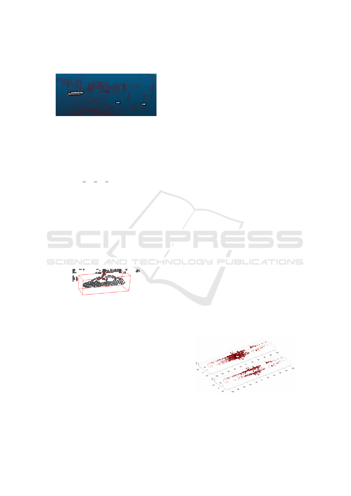
contains buildings but as shown in Figure 1 there is a
lack of labels for these objects.
Figure 1: Section of a H3D scenario with labels.
The labels have information about the center co-
ordinates of the object (x
0
, y
0
, z
0
), the length in ev-
ery coordinate direction (l
x
,l
y
,l
z
), and the yaw, so it is
possible to construct a 3D bounding box for each la-
beled object. The bounding boxes are constructed by
defining 8 new points (x
new
, y
new
, z
new
) - the corner co-
ordinates of a parallelepiped, which are computed as
(x
1
, y
1
, z
1
) = (±
l
x
2
, ±
l
y
2
, ±
l
z
2
). It is necessary to con-
sider the yaw angle (κ) in order to obtain the bound-
ing box with the proper orientation, so the new point
coordinates are computed by equation (13) using a 3D
rotation matrix:


x
new
y
new
z
new


=


cos(κ) −sin(κ) 0
sin(κ) cos(κ) 0
0 0 1




x
1
y
1
z
1


+


x
0
y
0
z
0


(13)
As an example, Figure 2 shows a car with the ap-
propriate reference bounding box.
Figure 2: Example of a Bounding Box reference for a car.
External validation indexes require the use of the
available labels, and to compute the index values it
is necessary to count the number of points inside a
bounding box. In order to facilitate index calcula-
tion, a new reference coordinate system is established.
The point cloud’s original center is translated to the
bounding box center, and the inverse rotation is ap-
plied as indicated in Equation (14), where (x, y, z) uses
the original coordinates of a data point, and (x
′
, y
′
, z
′
)
the new coordinates.


x
′
y
′
z
′


=


cos(−κ) −sin(−κ) 0
sin(−κ) cos(−κ) 0
0 0 1




x
y
z


−


x
0
y
0
z
0


(14)
5 RESULTS
The clustering results obtained for the H3D and
BOSCH datasets were treated separately since only
H3D has ground truth data.
5.1 H3D
In order to test the performance of the clustering
methods, five different scenarios were selected from
the LiDAR data. Scenario 1 corresponds to a traffic
scene with only one street recorded with several ve-
hicles and pedestrians circulating. Scenario 2 is very
similar to scenario 1 but it includes an intersection.
Scenario 3 corresponds to a road with several parked
cars near the sidewalk, very close to each other. Sce-
nario 4 is very similar to scenario 3 but it also includes
several cars on the road. Scenario 5 corresponds to an
intersection with a traffic light.
Before the application of the clustering algo-
rithms, it was necessary to pre-process the data to re-
move the ground. This is an important step because
firstly, the goal is not detecting the ground plane, and
secondly, the ground points connect separate objects,
such as cars and pedestrians, so it can affect the clus-
tering process. By removing the ground plane, there
will be fewer points to allocate, resulting in better-
separated objects. Consequently, it becomes easier to
identify obstacles and visualize clusters.
The method used for ground extraction was the
M-estimator SAmple Consensus (MSAC) algorithm
which is a variant of the RANdom SAmple Consen-
sus (RANSAC) algorithm (Azam et al., 2018). The
objective is to fit a plane to the point cloud data that
will contain the ground points denominated as inlier
points. The outliers are the points that do not belong
to the plane, thus the interest points for clustering. As
an example, Figure 3 shows the original point cloud
data for scenario 1 (top) and the points remaining af-
ter the ground removal process (bottom), indicating
that the ground removal procedure was successful.
Figure 3: Point cloud data for scenario 1: original (top);
after the removal of ground points (bottom).
In order to apply DBSCAN it is necessary to
choose values for the parameters m and ε (section
ICPRAM 2023 - 12th International Conference on Pattern Recognition Applications and Methods
826

2.2). Since the dataset is 3-dimensional, the suitable
value for m is 6. Figure 4 illustrates how to select the
appropriate ε, which for scenario 1 was found to be
0.7 since that is the value where the curvature of the
graph occurs. From that point onwards, the slope of
the graph becomes very high (near vertical).
Figure 4: Selection of the best value for ε (0.7), with m=6
for scenario 1.
Although the two algorithms were tested in 5 sce-
narios, only some results are presented graphically.
Figure 5 shows the results of DBSCAN on a data sec-
tion from scenario 1. A total of 167 clusters were
detected and 832 data points were classified as noise
(3.1%). Observing Figure 5, it is possible to conclude
that the method efficiently forms the clusters accord-
ing to the objects observed by the LiDAR. However,
as can be seen in the Figure, obstacles very close
to each other were not always divided into separate
groups. In scenario 4 this problem also occurs, since
DBSCAN grouped the parked cars in a single cluster
when it should have separated the cluster accordingly
to the number of parked vehicles. Figure 6 shows the
results of DBSCAN on a section of scenario 4, where
it is possible to observe this issue. In fact, in the sce-
narios in which the objects on the road are more dis-
tant from the sidewalk (such as scenario 2), the clus-
ters were better established, as illustrated in Figure 7.
However, in all the scenarios tested, in areas distant
from the sensor, the algorithm classified the points as
outliers, meaning that they do not belong to a cluster
since they are not dense enough to be identified as an
object.
Figure 5: DBSCAN clusters for scenario 1.
For every scenario tested, K-means was per-
formed with K equal to the number of clusters re-
turned by DBSCAN. It was verified that K-means
Figure 6: DBSCAN clusters for scenario 4.
Figure 7: DBSCAN clusters for scenario 2.
clustering did not perform as well as DBSCAN. This
was expected because K-means is a method based on
distance instead of density. For all tested scenarios, it
was possible to see that the method divided most ob-
jects into two or more clusters. This could be a result
of choosing a too-high value for K. However, even
when a smaller value for K is used, the algorithm still
performs poorly because it aggregates objects that are
clearly different and should thus be assigned to sepa-
rate clusters.
5.1.1 Internal Validation
Both methods (DBSCAN and K-means) grouped the
objects observed by LiDAR in several clusters, which
in some cases can be verified visually. However, in or-
der to extract meaningful information it is essential to
evaluate the results quantitatively. This is done using
both internal and external indexes. Table 1 presents
a summary of the internal indexes results, for all sce-
narios tested. It shows that for DBSCAN, the Silhou-
ette index is very low for all 5 scenarios, especially
in comparison with the values obtained for K-means.
In order to analyze these results, Figure 8 shows a
histogram with the Silhouettes index values for ev-
ery point in the data, for all the scenarios, using DB-
SCAN. The histogram shows that many points have a
negative I
S
value, which indicates that these points are
wrongly assigned to their cluster. In fact, for scenario
1, 35% of the data points have a negative I
S
value
and 68% have a value below 0.5. In order to identify
the points where the index performed poorly, Figure
9 shows the point cloud data for scenario 1 split into
2 groups: the points with I
S
< 0 (top) and with only
the points with I
S
≥ 0 (bottom).
Observing Figure 9, it becomes clear that the
points with I
S
< 0 correspond essentially to the ver-
tical walls in this scenario. This can be a result of
I
S
performing better with spherical clusters which is
not the case with walls. In fact, the clustering process
was repeated for scenario 1 with most of the walls re-
Clustering LiDAR Data with K-means and DBSCAN
827

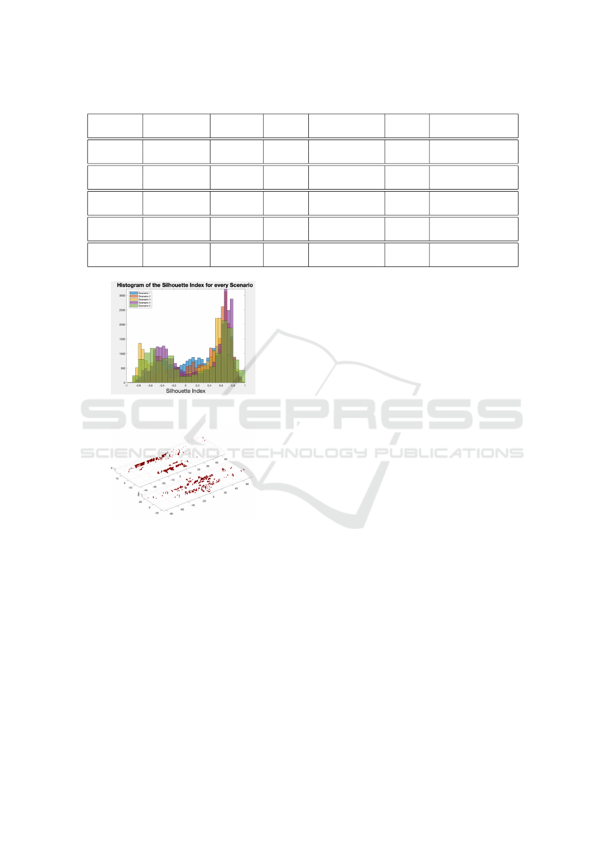
Table 1: Summary of internal indexes results for 5 test scenarios.
Scenario Method Silhouette Dunn Davies-Bouldin C-index Calinski–Harabasz
[Range];ideal [-1,1];1 [0,∞];∞ [0,1];0 [0,∞];0 [0,∞];∞
Scenario 1 DBSCAN 0.17 0.00359 0.59 0.0347 4645
K-Means 0.48 0.00135 0.72 0.0021 58025
Scenario 2 DBSCAN 0.35 0.00586 0.57 0.0125 9063
K-Means 0.53 0.00162 0.68 0.0019 59015
Scenario 3 DBSCAN 0.07 0.00269 0.66 0.0724 1967
K-Means 0.50 0.00269 0.68 0.0017 53211
Scenario 4 DBSCAN 0.21 0.00602 0.56 0.0310 4020
K-Means 0.49 0.00001 0.70 0.0026 55509
Scenario 5 DBSCAN 0.13 0.00481 0.69 0.0518 2615
K-Means 0.51 0.00481 0.65 0.0027 41809
Figure 8: Silhouettes Index values Histogram for DB-
SCAN.
Figure 9: Point cloud data split for scenario 1: points with
I
S
<0 (top) and with I
S
≥0 (bottom).
moved from the scene (using the same method applied
for ground removal), and the overall Silhouette’s co-
efficient changed from 0.17 to 0.29 for DBSCAN and
from 0.48 to 0.52 for K-means.
The Dunn’s Index for DBSCAN was higher for
K-means, in all scenarios tested, suggesting a better
performance for DBSCAN. However, the values are
all rather low, suggesting a poor performance.
The Davies-Bouldin validation index should have
a value close to zero to indicate good clustering re-
sults. However, the results in Table 1 present rather
high values, for all scenarios. Despite this, the I
DB
value is usually lower for DBSCAN than for K-
means. A more detailed analysis showed that for sce-
nario 1, DBSCAN had 20 clusters (out of 167) with
I
DB
value below 0.3, whereas K-means only had 3
clusters with I
DB
< 0.3.
Table 1 also shows the average C-index and
Calinski-Harabasz index. Both indicate better per-
formance for K-means clustering since they return
lower/higher (C-index/Calinski-Harabasz index) val-
ues for all scenarios.
Table 1 shows that for most internal validation in-
dexes, the values for DBSCAN are far from what was
expected. Accordingly to (Moulavi et al., 2014), these
indexes were created for evaluating convex-shaped
clusters (spherical clusters) and failed when applied
to validate clusters with arbitrary shapes. Therefore,
since the objects detected by LiDAR have different
forms and arbitrary shapes, the indexes presented are
perhaps not the most suitable ones to evaluate DB-
SCAN clustering results. For this purpose, (Moulavi
et al., 2014) proposes the DBCV index presented in
section 3.1.4. However, the DBCV is very demand-
ing computationally, so it can only be applied to small
data subsets.
In the interest of completing the clustering analy-
sis, DBSCAN was performed with different values for
m and ε to ensure that the choice of values for these
parameters was properly done. For scenario 1, the op-
timal value for ε was found to be 0.7 (the same value
obtained by analyzing Figure 4) since it produced the
highest I
S
value. Also, it was verified that as the value
of m increased, I
S
also increased. Similar results were
obtained for the other test scenarios.
The analysis of K-means clusters shows that most
objects were divided into several clusters suggesting
that the K value was too high. However, tests per-
formed with K between 1 and 167, for scenario 1,
did not improve the results considerably (I
S
values be-
tween 0.37 and 0.50).
ICPRAM 2023 - 12th International Conference on Pattern Recognition Applications and Methods
828

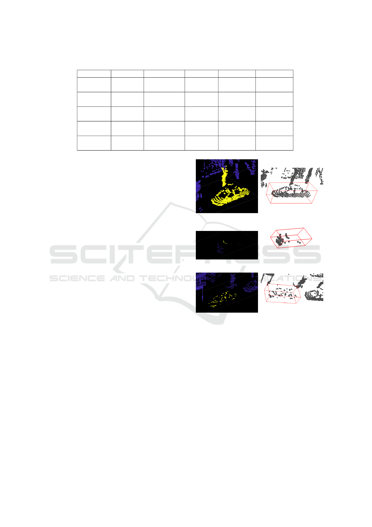
Table 2: Summary of external indexes results (range 0-1, where 1 is the ideal value).
Scenario Method Cluster Index Box Index Label Index CEVI Index
Scenario 1 DBSCAN 0.80 0.68 0.57 0.42
K-Means 0.79 0.83 0.38 0.31
Scenario 2 DBSCAN 0.94 0.91 0.72 0.67
K-Means 0.97 0.59 0.94 0.73
Scenario 3 DBSCAN 0.79 0.73 0.71 0.54
K-Means 0.77 0.52 0.64 0.41
Scenario 4 DBSCAN 0.91 0.99 0.37 0.35
K-Means 0.90 0.65 0.77 0.60
Scenario 5 DBSCAN 0.78 0.99 0.38 0.34
K-Means 0.62 0.84 0.38 0.28
5.1.2 External Validation
External indexes were calculated to complete cluster
validation using the procedure and the labeled data
described in section 4.2. Table 2 shows the Cluster,
Box, and Label indexes as well as CEVI, for both
methods in all test scenarios. The values presented in
Table 2 indicate that for the Cluster Index, the differ-
ence between K-means values and DBSCAN values
is relatively low, in 4 out of 5 scenarios. In scenario
5, DBSCAN outperformed K-means with a meaning-
ful difference between both values. On the opposite,
for the Box Index, there are considerable differences
in DBSCAN values and K-means values for all the
scenarios tested. DBSCAN proved to be better in 4 of
these scenarios. The Label Index values indicate that
each clustering method, outperformed the other in 2
scenarios, in scenario 5 their performance was equal.
The CEVI Index values suggest that in some scenar-
ios most of the labeled objects were not assigned to
a cluster since the value for the index was rather low
(scenarios 1 and 5). In addition, DBSCAN performed
better than K-means in scenarios 1,3,5, although the
values were unsatisfactory.
In order to obtain a more detailed analysis, three
objects from scenario 1 were selected for a thor-
ough inspection. Figure 10 illustrates the three typ-
ical cases that occur: a cluster joining two different
objects (IE
C
< 1), the clustering method dividing an
object into two or more clusters (IE
B
< 1), and the
ideal case where the cluster corresponds to the object
(IE
C
= 1, IE
B
= 1). IE
C
is responsible for measuring
if the number of points in a cluster matches the num-
ber of points inside the associated reference bounding
box. Therefore, IE
C
< 1 occurs whenever a cluster
joined two or more different objects. Figure 10 (a-
b) shows an example of the first situation. DBSCAN
joined two different objects in a unique cluster lead-
ing to a IE
C
value of 0.75 (< 1). However, the Box
Index value was equal to one because the object with
the labeled car is all in the cluster. Another typical
(a) IE
C
= 0.75 IE
B
= 1.00
(b) Bounding box Cluster 50
(c) IE
C
= 1.00 IE
B
= 0.13 (d) Bounding box Cluster 82
(e) IE
C
= 1.00 IE
B
= 1.00 (f) Bounding box Cluster 44
Figure 10: Typical cases (from scenario 1) for external in-
dexes values with the reference bounding boxes.
case occurs when IE
B
< 1. This case happens when
#C
bbx
< #BB
x
meaning that the cluster divides an ob-
ject into two or more clusters. Figure 10 (c-d) shows
an example where the entire cluster is inside the ob-
ject bounding box, but the cluster did not allocate all
the object points, justifying the low value for IE
B
. The
ideal case occurs when the cluster matches the object
(IE
C
= 1, IE
B
= 1), as the example shown in Figure
10 (e-f).
To complete the detailed analysis of the DBSCAN
clustering for scenario 1, Table 3 shows some relevant
information about the labeled clusters: the cluster id,
the associated label, the number of points belonging
to the cluster, the within-cluster variance and the dis-
tance of the cluster to the LiDAR sensor. Table 3 in-
Clustering LiDAR Data with K-means and DBSCAN
829

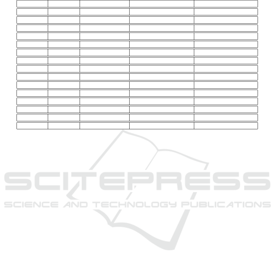
Table 3: Summary of the detailed analysis of DBSCAN clusters from scenario 1.
Cluster Id Label Number of Points Within Cluster Variance Distance to LiDAR (m)
12 Truck 10 2.80 35.53
25 Car 6 0.38 23.036
31 Pedestrian 142 44.81 11.39
44 Car 116 215.42 8.21
50 Car 390 859.68 12.10
57 Pedestrian 19 2.41 22.36
66 Car 261 874.64 21.52
82 Car 6 0.46 28.76
103 Car 15 2.97 17.16
104 Car 43 7.54 15.66
109 Pedestrian 26 2.57 15.13
113 Pedestrian 15 1.00 12.29
121 Pedestrian 214 21.86 6.20
152 Pedestrian 57 9.72 18.37
154 Car 85 117.48 11.98
dicates that clusters corresponding to vehicles have a
larger point dispersion than pedestrian clusters. For
example, cluster 66 corresponds to a car and has 261
points with a (V
WC
) value of 874.64, whereas cluster
121 corresponds to a pedestrian with nearly the same
number of points (214) and has a (V
WC
) value of only
21.86. Thus, it is possible to conclude that pedestri-
ans form clusters with lower dispersion than vehicles.
Furthermore, the Distance to the LiDAR is meaning-
ful information since these values indicate how close
an object is to the vehicle. For the scenario 1 test case,
the pedestrian in cluster 121 is the closest object to the
LiDAR sensor.
5.2 BOSCH Data
Only one test scenario from the BOSCH data was se-
lected, corresponding to a section of a highway with a
bridge and large areas of vegetation on the sides. Be-
fore applying the clustering methods, ground removal
was performed using a similar procedure as for H3D
data. The analysis of this test scenario allows the dif-
ferences between data collected from urban areas and
highways to be seen.
DBSCAN returned a total of 270 clusters with
1786 data points classified as noise (0.8055%). This
scenario presented fewer objects and large areas of
vegetation on both sides, so there were not many ob-
jects to segment. In fact, the variety of clusters de-
tected by DBSCAN in vegetated areas was consid-
ered of low interest. Nevertheless, DBSCAN effi-
ciently clustered the bridge presented in the scenario.
Similar to what was verified for H3D, K-means per-
formed poorly in regard to the visual interpretation,
since the method divided a single object into different
clusters. The K-means clustering procedure was re-
peated for several values of K, and the optimal value
for K proved to be 3. This resulted in an average
silhouette value of 0.78. However, the clusters did
not correspond to the objects observed by the LiDAR
since with only 3 clusters the method joined several
objects into the same cluster.
In order to evaluate the clustering results from
both clustering methods (DBSCAN and K-means),
the internal validation indexes presented in section
3.1 were computed. However, the results for all in-
dexes were unsatisfactory, especially for DBSCAN.
DBSCAN presented a negative value for the silhou-
ette’s index indicating that most points were wrongly
assigned to their cluster. K-means outperformed DB-
SCAN in every index with a I
S
value of 0.39, I
DB
of
0.80, and I
CH
of 580940. For both clustering methods,
it was not possible to calculate the Dunn Index and
the C-index because the data includes 771120 points
(almost seven times more than H3D scenarios).
The analysis of the BOSCH data confirmed that
K-means performs better than DBSCAN in most in-
ternal indexes but this is not confirmed by a visual
interpretation where in fact it performs worst.
6 CONCLUSIONS
The purpose of the two clustering methods presented
in this paper is to extract information from large Li-
DAR datasets. Grouping data into clusters enables
object detection and further classification, which can
improve the safety of autonomous driving vehicles.
ICPRAM 2023 - 12th International Conference on Pattern Recognition Applications and Methods
830

The clustering experiment carried out, indicated
that DBSCAN is more effective than K-means since
it detected arbitrary cluster shapes. In addition, DB-
SCAN performed better than K-means in the Dunn
Index (I
D
) (higher values of I
D
) and in the Davies-
Bouldin Index (I
DB
) (values closer to 0), in most of
the scenarios tested. Despite this, the values were not
very good, which might indicate that these indexes
are not the best suited to validate clusters with ar-
bitrary shapes. K-means outperformed DBSCAN in
Silhouette’s index (values closer to 1), C-index (val-
ues closer to 0), and Calinski-Harabasz (higher val-
ues of I
CH
). The detailed analysis of Silhouette’s in-
dex indicated that the points with lower I
S
values cor-
respond mostly to walls/buildings, which are objects
that do not have a spherical shape. Thus DBCV index
is the appropriate index to validate clusters with arbi-
trary shapes. Despite this, the index is very demand-
ing computationally to apply to the complete dataset.
This index is only suitable for small data subsets.
The experiment with five H3D test scenarios leads
to the conclusion that DBSCAN performs better when
the objects in the scene are rather distant. For objects
very close to each other, DBSCAN clustered different
objects into the same cluster.
The ground removal procedure proved to be an es-
sential requirement to separate the interest objects in
all scenarios tested. The method presented to con-
struct the reference bounding boxes for H3D objects
proved efficient and essential to compute the exter-
nal validation indexes. Regarding these indexes, DB-
SCAN performed better than K-means in the basic ex-
ternal indexes, in most test scenarios. The Composite
External Validation Index (CEVI) evaluated the over-
all results from Cluster, Box, and Label indexes, and
DBSCAN outperformed K-means in 3 of the scenar-
ios tested. The detailed analysis of DBSCAN clus-
ters indicated that pedestrian clusters have a low value
for the within-cluster variance (V
WC
). Therefore these
clusters have smaller dispersion than the vehicles
clusters. The analysis of H3D and BOSCH datasets
led to the conclusion that DBSCAN and K-means are
more useful in urban scenarios than in highway sce-
narios since there are more objects to cluster.
As a final remark, it can be concluded that clus-
tering methods are a useful technique for segmenting
LiDAR data. Further work should include research
on appropriate internal validation indexes to validate
arbitrarily shaped clusters for all sorts of dataset sizes.
ACKNOWLEDGEMENTS
This work is supported by European Structural
and Investment Funds in the FEDER component,
through the Operational Competitiveness and Interna-
tionalisation Programme (COMPETE 2020) [Project
nº 047264; Funding Reference: POCI-01-0247-
FEDER-047264].
REFERENCES
Arbelaitz, O., Gurrutxaga, I., Muguerza, J., P
´
erez, J. M.,
and Perona, I. (2013). An extensive comparative
study of cluster validity indices. Pattern Recognition,
46(1):243–256.
Azam, S., Munir, F., Rafique, A., Ko, Y., Sheri, A. M., and
Jeon, M. (2018). Object modeling from 3d point cloud
data for self-driving vehicles. In 2018 IEEE Intelligent
Vehicles Symposium (IV), pages 409–414.
Ester, M., Kriegel, H.-P., Sander, J., Xu, X., et al. (1996).
A density-based algorithm for discovering clusters in
large spatial databases with noise. In kdd, volume 96,
pages 226–231.
Halkidi, M., Batistakis, Y., and Vazirgiannis, M. (2001). On
clustering validation techniques. Journal of intelligent
information systems, 17(2):107–145.
Moulavi, D., Jaskowiak, P. A., Campello, R. J. G. B.,
Zimek, A., and Sander, J. (2014). Density-based clus-
tering validation. In SDM.
Patil, A., Malla, S., Gang, H., and Chen, Y.-T. (2019). The
h3d dataset for full-surround 3d multi-object detection
and tracking in crowded urban scenes. In Interna-
tional Conference on Robotics and Automation.
POCI-01-0247-FEDER-047264. Project nº 047264.
Ramos, J. (2022). Dunn’s index. MATLAB Central File
Exchange. Retrieved September 7, 2022.
Sander, J., Ester, M., Kriegel, H.-P., and Xu, X. (1998).
Density-based clustering in spatial databases: The al-
gorithm gdbscan and its applications. Data mining
and knowledge discovery, 2(2):169–194.
Syakur, M., Khotimah, B., Rochman, E., and Satoto, B. D.
(2018). Integration k-means clustering method and
elbow method for identification of the best customer
profile cluster. In IOP conference series: materials
science and engineering, volume 336, page 012017.
IOP Publishing.
Wang, C., Ji, M., Wang, J., Wen, W., Li, T., and Sun, Y.
(2019). An improved dbscan method for lidar data
segmentation with automatic eps estimation. Sensors,
19(1):172.
Xu, D. and Tian, Y. (2015). A comprehensive survey
of clustering algorithms. Annals of Data Science,
2(2):165–193.
Clustering LiDAR Data with K-means and DBSCAN
831