Outlier Detection Method for Equipment Onboard Merchant Vessels

Iori Oki

, Seiji Yamada

2 b

and Takashi Onoda

1 c

Aoyama Gakuin University School of Science and Engineering, 5-10-1 Huchinobe, Chuo, Sagamihara, Kanagawa, Japan

National Institute of Informatics 2-1-2 Hitotsubashi, Chiyoda, Tokyo, Japan

Keywords:

Anomaly Detection, Outlier Detection, Explainable AI, Explainability, One-Class Support Vector Machine,

SHAP.

Abstract:

The equipment onboard merchant vessels are essential for safe navigation. If an equipment malfunction occurs

during a voyage, it is difﬁcult to repair it with the same speed and accuracy as on land. Therefore, it is important

to It is required to be able to repair and replace the equipment with a margin of time by detecting the signs

of anomalies. In this paper, we present the results of detecting signs of anomalies from various sensor data

collected using One-Class SVM. It also show s the results of interpreting the signs of anomalies and detected

locations using SHAP. The results show that the proposed method can detect signs of anomalies at a point

about one month before the conventional method. Therefore, the proposed method is shown to be potentially

useful for the maintenance of equipment on merchant vessels.

1 INTRODUCTION

In recent years, to maintain schedules and ensure safe

operations, efforts have been made not only to main-

tain and manage safe vessel operations, but also to

ensure safe navigation and marine envir onment con-

servation from various perspectives. To maintain safe

vessel operation, it is important for navigators to con-

duct proper monitoring and to select the best route in

consideration of weather and sea conditions. In the

engine room, the condition of the main engine, which

propels the ship, and auxiliary engines, such as mo-

tors, which are important for operation, are monitored

by the engineer, and preventive maintenance manage-

ment is conducted. To prevent severe damage, these

devices are repaired o r replace d when anomalies are

detected during daily patrol inspections of their op-

erating conditions. Traditionally, vessel monitoring

equipment has been minimal and inspections have re-

lied on the human senses. In recent years, with the im-

provement of technology such as temperature, pres-

sure, and vibra tion sensors, there have been efforts to

detect anomalies through automatic mo nitoring, but it

is still insufﬁcient. Ship equipment is characterized

by the fact th at once it goes out to sea, it does not

return for a long period of time and that repair s that

https://orcid.org/0000-0001-7617-6000

https://orcid.org/0000-0002-5907-7382

https://orcid.org/0000-0002-5432-0646

can be done easily on land are difﬁcult to do at sea.

Therefore, events tha t would be detected on land in

time after an a nomaly is detected must be detected

and responded to before that time for vessels.

In this paper, we describe related research in the

next section. In the section 3, w e explain the sub-

ject data. In the section 4, we brieﬂy explain section

the proposed method of detecting signs of anoma lies

in equipment onboard merchant vessels. The exper-

imental results are shown in the section 5. Finally,

we conclude the concept of anomaly pre diction detec-

tion f or equipment onboard merchant vessels based

on outlier detection methods.

2 RELATED RESEARCH

In the marine ﬁeld, monitorin g the condition of equip-

ment and achieving condition-based maintenance is

still a new study. In the past few years, studies

have bee n conducted in supe rvised learning. (Porteiro

et al., 2011) presented a multi-net fault diagnosis sys-

tem to provide power estimation and fault identiﬁca-

tion of a diesel engine. (Coraddu et al., 2016) pro-

posed an app lica tion of supervised machine learn-

ing approaches to estimate the decay status of a

naval propulsion plant for improving condition based

maintenan ce. (Cipollini et al., 2018b) and (Cipollini

et al., 2018a) proposed some supervised and unsuper-

Oki, I., Yamada, S. and Onoda, T.

Outlier Detection Method for Equipment Onboard Merchant Vessels.

DOI: 10.5220/0011665300003411

In Proceedings of the 12th International Conference on Pattern Recognition Applications and Methods (ICPRAM 2023), pages 649-660

ISBN: 978-989-758-626-2; ISSN: 2184-4313

 2023 by SCITEPRESS – Science and Technology Publications, Lda. Under CC license (CC BY-NC-ND 4.0)

649

vised approaches for condition based maintenance of

a naval gas propulsion plant. (Lazakis et al., 2019) in-

vestigated a One-Class supp ort vector machine (One-

Class SVM) based approach to realize condition mon-

itoring of a marine diesel gener a tor with the noon-

report data. (Brandsæter et al., 2019) developed an

on-line anom aly detectio n approach based on mul-

tivariate signal reconstruction followed by residuals

analysis for anomaly detection of a marine diesel en-

gine in operation. Supervised learning algo rithms

have been proposed fo r condition monitorin g of ma-

rine equipmen t systems. However, (Tan et al., 2020)

said that supervised learning algorithms tend to be

unrealistic, because the fact that most of the sam-

ples mo nitored by the shipb oard monitoring system

are normal samples is ignored and the required la-

beled samples are not easy to o btain. They pro-

posed the use of a one-class classiﬁcation technology.

Speciﬁcally, a comparative study of Condition moni-

toring of the marine equipment system was conducted

using six one-class classiﬁcation algorithms: One-

Class SVM, Support vector data description (SVDD),

Global k-nearest neighbors (GKNN), Local outlier

factor (LOF), Isolation Forest (IForest), and Angle-

based outlier detec tion (ABOD). The results show

that the one-class classiﬁcation algorithm is applica-

ble to marine equ ipment.

However, when it comes to actual use in the ﬁeld,

a system that only detects signs of anomaly not be

adopted by companies. The reason is that it does not

explain what the cause of the problem is. In recent

years, the ﬁeld of Explainable AI has ﬂourished, as

can be seen from Figure 1. From ﬁgure 1, we can

see that companies ar e demanding evidence for the

results of machine learning. In other words, by pro-

viding clear evidence f or detection results, companies

are expected to be more proactive in detecting anoma-

lies usin g machine learning.

In this study, the one- class classiﬁcation algorithm

was applied to merchant marine equipment to ver-

ify whether it is possible to de tect predictive signs

of anomalies. In addition, we use SHAP, one of the

interpretation methods o f the one-class classiﬁcation

algorithm , to clarify the basis for the detection of pre-

dictive signs of anomaly.

3 MEASUREMENT DATA

In this study, under the collaboration with Furuno

Electric Co. we will detect predictive signs of anoma-

lies in equipment onboard merchant ships. Data from

equipment onboard merchant vessels is sent via satel-

lite to a data center on land. The n, the data center

Figure 1: Explainable AI Papers by Year (Adadi and

Berrada, 2018).

detects signs of anomalies, and if an anomaly is con-

ﬁrmed, instructions are given for repair or rep la c e-

ment. So, note that we do not perform predictive

anomaly detection within the merchant vessel. In the

3.1 section, describes the target equipment onboard

merchan t vessels, and describes the data of the target

equipment in the 3.2 section.

3.1 Equipment Onboard Merchant

Vessels

There are several types of equipment onb oard mer-

chant vessels, each of which plays a key role in e n-

suring safe navigation. For example, acoustic depth

gauges measure the depth of the water, which is im-

portant to avoid running aground . Other devices in-

clude satellite spee d logs that provide information on

the speed of merchant vessels, which is indispens-

able when berthing. Among these various devices,

this study focuses on the common parts of the devices

called Radar and ECDIS (see Figur e 2). A ra dar is a

device that uses the bounce of radio waves to check

the movement of other vessels and to conﬁrm the

safety of the surroundings. It is especially effective

when visibility is poor due to rain or snow and is an

especially important device that can hinder the safety

of navigation if it is broken. The other is ECDIS,

which digitizes and displays paper charts to create

ship routes. This is another important piece of equip-

ment that must be equipped. Although there are many

target devices, we selected one o f them for this exper-

iment. The selection criteria are individuals selected

by the experts of Furuno Electric Co. from among

equipment whose sensor values were measured to be

anomaly.

ICPRAM 2023 - 12th International Conference on Pattern Recognition Applications and Methods

650

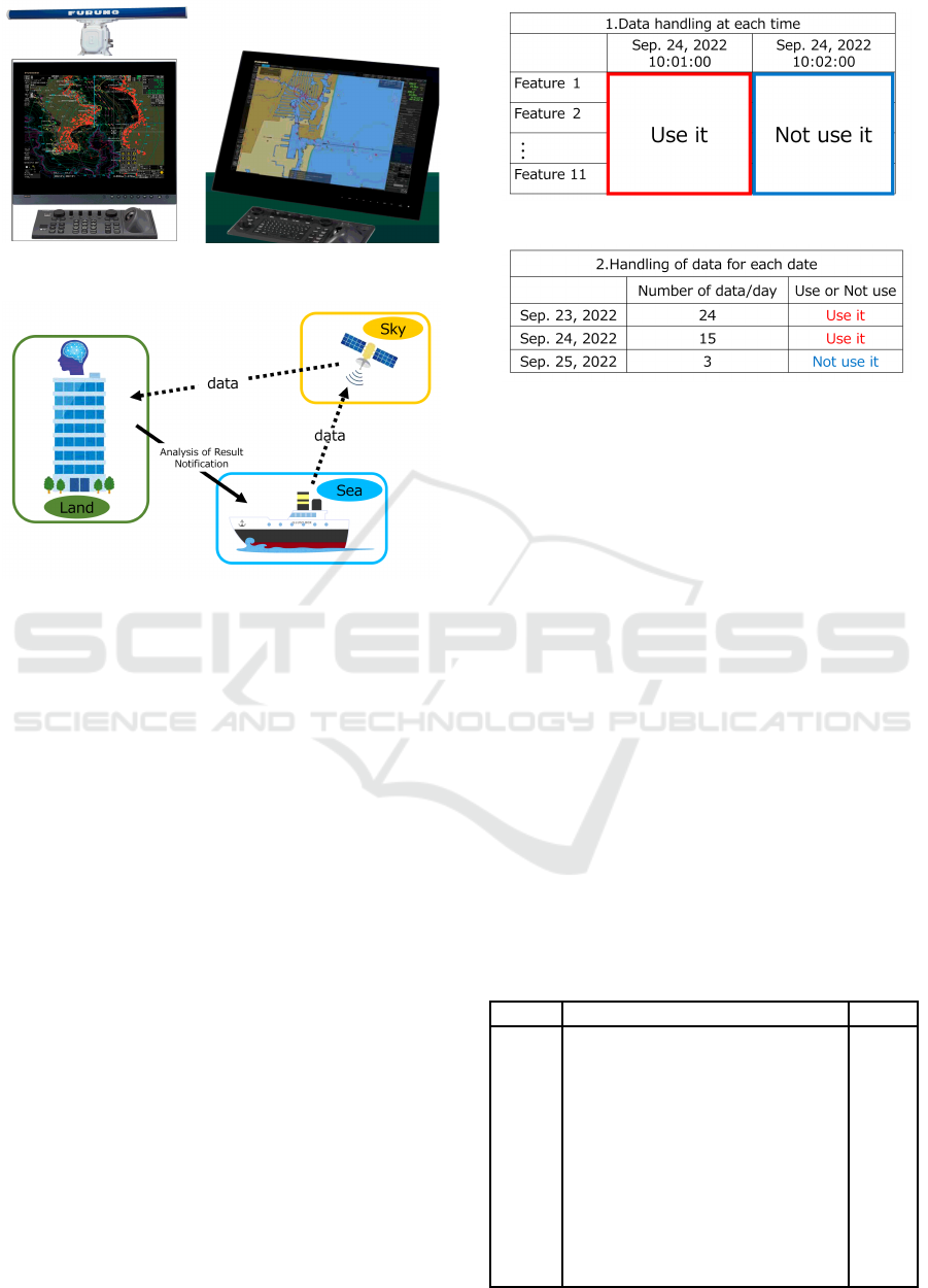
Figure 2: Equipment on board merchant vessels; left:

Radar, Right:ECD IS.

Figure 3: Data ﬂow.

3.2 Used Data

The data of the target equipment described in sec-

tion 3.1 is acquired as shown in Figu re3. Sensor val-

ues recorded o n the merchant vessel are collected via

satellite to a data cen te r locate d on land. One case

of data is obtained every hour. Anomaly detection

is the n performed at the data center where the data

was collected, and if an anomaly is conﬁrmed, the

merchan t vessel carrying the a nomalous individual is

contacted. The contacted merchan t vessel will take

action, suc h as repairing the anomaly or re placing it

with a spare piece of equipment on board, depend-

ing on the extent of the anomaly. However, some of

the data contain missing data or errors due to satellite

communication problems. Therefore, the acquired

data cannot be used fo r experiments as is. T herefor e,

to address this issue, two data use conditions were

established in this study based on expert advice and

analysis.

1. If multiple data are acquired in one hour, the ﬁrst

acquired data is used because the later data is error

data (Fig ure 4).

2. If the con ditions in 1. are met and the total number

of data acquired in a day is less th an 15, the data

for that day not be used (Figure 5).

The eleven sensors used are listed in the Table 1.

These are all senso rs that the subject equipment can

Figure 4: Data Use Condition(time).

Figure 5: Data Use Condition(day).

acquire. These 11 items are currently used by on-site

inspectors to conduct inspections, so we used these

same condition s. The subject individuals had a total

of 26,425 data that met the conditions of use, and the

acquisition period was from December 2015 to Febru-

ary 2019.

4 ANOMALY PREDICTION

DETECTION METHOD

In this section, we describe a mod el for detecting pre-

dictive signs of anomalies in equipment o nboard mer-

chant vessel. This study uses One-Class SVM, an out-

lier detection model, and the Mahalanobis-Taguchi

Method (M T Method), a statistical method.

4.1 One-Class SVM

One-Class SVM is an extension of the classical SVM,

and it is a common semi-supervised learning tech-

Table 1: Data Summary

Order Sensor I te m Units

1 CPU FAN RPM rpm

2 CPU FAN 1 RPM rpm

3 CPU FAN 2 RPM rpm

4 CPU board temperature degC

5 CPU Core Temperature degC

6 GPU Core Temperatu re degC

7 CPU core power supply voltage V

8 Battery sup ply voltage V

9 3.3V supply voltage V

10 5V sup ply voltage V

11 12V su pply voltage V

Outlier Detection Method for Equipment Onboard Merchant Vessels

651

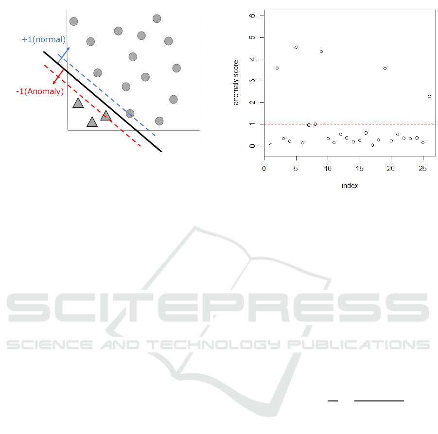
Figure 6: One-class SVM.

nology used to solve one-class classiﬁcation problem

(Khan and Madden, 2010). In the classical SVM,

it can determine an optimal hype rplane by maxi-

mizing the interval between the support vectors of

two classes. However, in One-Class SVM, there are

only one-class data points involved in model training,

which makes it impossible to ﬁnd the optimal hyper-

plane like the classical SVM. In fact, it regards the

origin as the only negative data point and all train-

ing data as po sitive points. The g oal of model train-

ing is to make the classiﬁcation hyper-plane as far

away from the origin as possible. After transform-

ing the feature via a kernel, they treat the origin as the

only member of the second class. The using relax-

ation parameters they separate the image of the one

class from the origin. The n the standard two class

SVM techniques are employed (Vapnik, 1999). One-

Class SVM (Sch¨olkopf et al., 2000) returns a fu nc-

tion of that takes the value +1 in a small region c ap-

turing most of the training data points, and -1 else-

where. The algorithm can be summarized as mapping

the data into a fe ature space using an appropriate ker-

nel function, and th e n trying to separa te the mappe d

vectors from the origin with maximum margin (see

Figure 6).

4.2 MT Method

The MT method, proposed by (Taguchi and Jugu-

lum, 2002), is a practica l method for anomaly de-

tection, developed from Hotelling’s T

control chart

(Hotelling, 1947) by adding ideas such as item selec-

tion and item diagnosis. The MT method assumes

that only nor mal data form a homogeneous popula-

tion. Then, if the new data does not deviate from the

formed population, it is judged as normal, and if it

does, it is judged as ano maly. This homogeneous pop-

ulation is called the unit space in the MT method. The

Figure 7: MT Method Sample.

measurement of deviate level from the unit space is

quantiﬁed based on the Mahalanobis distance. In ac-

tual use, a th reshold value is set in advance, and if the

value is exceeded, it is judged as anomaly (see Figure

7).

Another feature of the MT method is called

Signal-to-Noise (S/N) ratios. This quantiﬁes th e con-

tribution of individual variables and allows interpre-

tation of the results of the MT method as to what is

due to what. Taguchi empirically introduced an in-

dicator such as Equation 1, which is the S/N ratios

for the variable set q. Where M

in Equ a tion 1 rep-

resents the number of variables and a

represents the

anomaly when using a covariance matrix of M

× M

dimensions.

≡ −10log

{

′

∑

n=1

′(n)

)/M

} (1)

Calculating the S/N ratios in this way yields the con-

tribution of each variable as shown in Figure 8. Figure

8 shows the results for the road data included in the

MASS package, and the cities shown are in Califor-

nia. The S/N ratios ind ic ates that a large value is in-

ﬂuential. The results show that almost all of the large

anomalies in California are caused by fuel. Thus, the

MT method not only detects a nomalies, but also iden-

tiﬁes their causes by a unique method called the S/N

ratios.

5 CONTRIBUTION

CALCULATION METHOD

The MT m ethod has its own interpretation method

as described in section 4.2. On the other hand,

ICPRAM 2023 - 12th International Conference on Pattern Recognition Applications and Methods

652

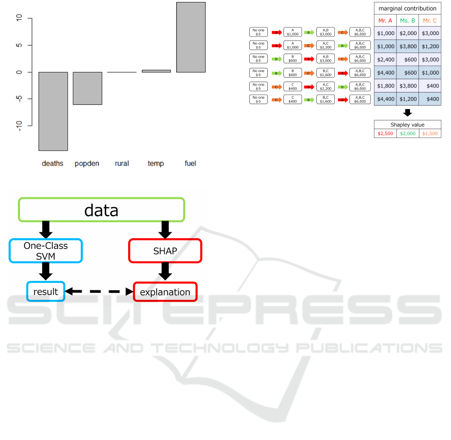
Figure 8: SN ratio Sample.

Figure 9: Relationship between One-Class SVM and SHAP.

One-Class SVM can be interpreted by using coefﬁ-

cient in the case of linear kernels, but there is no

such method for RBF kernels. Therefore, a differ-

ent approach must b e used for interpretation. Cur-

rently, DARPA, which conducts defense research in

the United States, categorizes Explainable AI ap-

proach e s into three broad categories(Gunning et al.,

2019). These three approaches are: feature v isu aliza-

tion, generation of interpretable models, and approx-

imation by interpretable models. In this study, we

interpret One-Class SVM models based on Shapley

additive explanations (SHAP), a type of f eature visu-

alization. The relationship between One-Class SVM

and SHAP is shown in Figure 9 SHAP uses the ma-

chine le a rning model and the data used in the model

to measure the contribution of each feature and to add

interpretability to the results of the machine learn ing

model. This SHAP was originally based o n the con-

cept of the Shapley value in cooperative game theory.

Therefore, this chapter describes the Sh apley value

and SHAP.

Figure 10: Shapley.

5.1 Shapley Value

In cooperative game theory, the Shapley value is a

means used to fairly distribute the beneﬁts in a game

in which multiple players cooperate, according to

each player’s contribution. As an example, suppose

we have a situation in which different people partici-

pating in a game receive different rewards. The list of

rewards is as follows.

• If only Mr. A participates, the compensatio n is

$1,000.

• If only Ms. B p articipates, the compensation is

$600.

• If only Mr. C participates, the compensation is

$400.

• If Mr. A and Ms. B participate, the reward will be

$3,000 for both of them.

• If Ms. B and Mr. C participate , the reward will be

$1,600 for both of them.

• If Mr. A and Mr. C participate, the reward will be

$2,200 for both of them.

If the rewa rd for p articipation by Mr. A, Ms. B, and

Mr. C is $6,000, consider the question of how fairly

to divide the reward among Mr. A, Ms. B, and Mr. C.

First, consider the situation where Mr. A participates

from a situation where no one else participates. Th is

raises the reward from $0 to $1,00 0. In other words,

we can say that Mr. A contributed to raising the re-

ward by $1,000 . Next, consider the situation where

Ms. B is participating and then Mr. A joins him.

In th is case, the compensation goes up from $600 to

$3,000, so Mr. A contributed to raising the reward

by $2, 400. This contribution is called the margina l

contribution, and the average of the marginal contri-

butions of all combinations is the Shapley value. In-

cidentally, in this example, it is fair to divide Mr. A,

Ms. B, and Mr. C into $2,500, $2,000, and $1,500, as

shown in Figu re 10.

Outlier Detection Method for Equipment Onboard Merchant Vessels

653

5.2 Shapley Additive

Explanations(SHAP)

SHAP is a machine learning application of the Shap-

ley values de scribed in Section 5.1. In SHAP, the

Shapley value represents the performance of a featur e

in the machine lea rning mod el. In other words, Mr. A,

Mr. B, and Mr. C used in the Shapley value example

represent each feature value in SHAP.

SHAP uses an additive feature attribution method,

i.e., an ou tput model is deﬁned as a linear addition of

input variables(Mangalathu et al., 2020). Assuming a

model with input variables x = (x

,... ,x

) where

p is the number of input variables, the explana tion

model g(x

′

) with simpliﬁed input x

′

for an original

model f (x ) is expressed as

f (x ) = g(x

′

) = φ

∑

i=1

′

(2)

where M r e presents the number of inpu t features, and

represents the constant value when all inputs are

missing. Inputs x

′

and x are related through a map-

ping function, x = h

′

). Equation 2 is illustrated in

Figure 11, where φ

, φ

, and φ

increase the pre-

dicted value o f g(), while φ

decreases the value of

g().

As noted by (Lundberg and Lee, 2017), a single

solution exists for Equation 2, which ha s three desir-

able properties: local accuracy, missingness, and con-

sistency. Local accuracy ensures that the outpu t of

the function is the sum of the fe ature attributions and

requires the model to match the output of f for the

simpliﬁed input x

′

. The loca l accuracy happens when

x = h

′

). M issingness ensures that no importance is

assigned to missing features. As φ

′

implies φ

= 0,

missingness is satisﬁed. Through the consistency,

changin g a larger impact fea ture will not decrease the

attribution assigned to that feature. For a setting z

′

when z

′

= 0, f

′

)− f

′

\i) ≥ f

′

)− f

′

\i) im-

plies φ

( f

′

,x) ≥ φ

( f ,x). The only possible model that

satisﬁes these properties is

( f ,x) =

∑

′

⊆x

′

|!(M − |z

′

| − 1)!

[ f

′

) − f

′

\i)]

(3)

where |z

′

| represents the number of non-zero entries in

′

, and z

′

⊆ x

′

, and φ

from Equation 3 is the Shapley

values. (Mangalathu et al., 2018) suggested a solution

to Equation 3 where f

′

= h

′

) = E[ f (z)|z

] and S

is the set of non-zero indices in z

′

, known as SHAP

values.

In this study, we decided to use this SHAP to cal-

culate the contribution to the anomaly detection loca-

tions. The reason for using SHAP is that SHAP is lo-

cally interpr etable. In the ﬁeld of anomaly detection,

we do not want to capture overall trends and evalu-

ate which sensors strongly inﬂuenced the model. It

is necessary to calculate the contribution of each and

every location that is determine d to be anomaly, and

to know and analyze under what kind of inﬂuence the

anomaly was determ ined in that location. We though t

SHAP desirable because it allowed us to calculate the

contribution one location at a time. When calculating

the contribution using SHAP, all that is needed is the

model and feature data from the prediction an d esti-

mation. In this study, the model to be passed to SHAP

is the One-Class SVM model, and the feature data is

the test data from the tests conduc ted on the model.

However, the te st data was limited to only those ar-

eas identiﬁed a s anomalies in the One-Class SVM

model. The speciﬁc contribution calculation method

is as shown in Figure 12. First, the One-Class SVM

model and the data of the location that was tested and

determined to be anomalies in the model are prepared.

Next, each contribution is c a lc ulated for each feature

of the data in the areas determined to be anomaly as

in Fig ure 13. The expression of not participating in

the Shapley value is replaced in SHAP with a value

of no impact using the predicted expected value. In

this way, the difference between when the feature is

affected and when it is unaffected can be calculated.

This is done in various combinations and averaged

to obtain the contribution. Since this stu dy targets

anomaly detection by the One-Class SVM model, the

contribution is based on the degree of anomaly, i.e.,

the distance from the o ptimal hyperplane.

6 EXPERIMENTAL RESULTS

In th is section, after describing the experimental con-

ditions, the results of the anomaly prediction de te c-

tion and contribution estimation experiments are pre-

sented.

6.1 Experimental Procedures

Section 6.1 describes the experimental conditions.

Please refer to Figure 14 as you read it. First, the

missing data are pr ocessed as describ e d in section 3.2.

Next, the 11 features for present use in the inspection

are selected. Next, extract the data periods to be used

in the model. In this case, as shown in Figure 15, one

month was used as test data and the last two years of

the test period as training data. The reason for this

setup is the re quest of the experts at Furuno Electric

Co. to update the model every month with respect to

the test data. A s for the training data, the experts and I

came to the conclusio n that using older data would be

ICPRAM 2023 - 12th International Conference on Pattern Recognition Applications and Methods

654

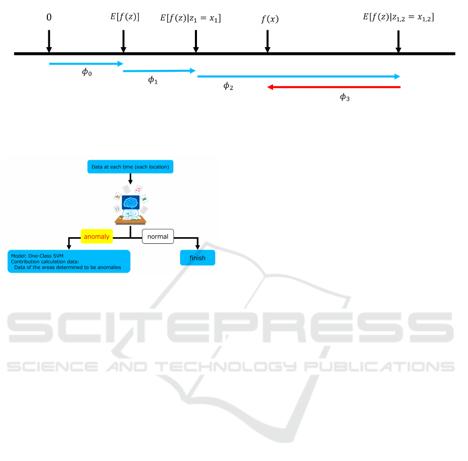
Figure 11: Example of SHAP with 3 variables(Lundberg and Lee, 2017). E[ f (x)] is the predicted value assuming all three

features were not observed. The measured values are then entered into the features one by one, and the movement of the

predicted values is measured as a contribution. In this example, we can see that x

and x

have a positive contribution and x

has a negative contribution.

Figure 12: Flow to SHAP.

affected by age- related deterioration, so we decided

to use two years. This means that the model was built

15 times in this study. The number of training data at

one time is approximately 17,000 and the number of

test data is approximately 700. Then, normalization is

performed, and models are constructed using training

data in each of the MT and One-Class SVM methods.

The constructed model is then used to detect anoma-

lies in the test data. Here, th e MT method r e quires a

pre-determined threshold value, but in this case, we

used 4 as a general guideline. One-Class SVM re-

quire a preconﬁgured kernel. In this study, a Radial

Basis Function (RBF) kernel was used. Therefore, it

is necessary to set the parameters ν and γ. ν was set

to 0.02. On the other hand, f or γ, we tried 0. 01, 0.1,

1.0, 10 and veriﬁed which γ value is optimal. After

the anomaly prediction detection exp e riment, we es-

timated the cause of the anomaly by usin g the S/N

ratios for the areas identiﬁed as an omalous b y the MT

method and SHAP for the areas identiﬁed as anoma-

lous by the One-Class SVM metho d.

6.2 Results of the Experiment for

Detecting Signs of Anomaly

Before presenting results of anomaly prediction de-

tection experiment, we will discuss the areas diag-

nosed as anomalies in terms of the data me ntioned

in section 3.1. Figu re 16 shows the time series graph

of CPU FAN2 RPM for the experiment. This clearly

shows that we have recorded something of an out-

lier in the late August 2018 data. When this data

was shown to the experts, the data recorded at 4:00

AM Japan time on August 2 5, 2018, was fo und to

be anomalou s. The goal is to detect this area a s an

anomaly and how to detect signs of anomalies further

down the road. We shall also refer to this part as the

defective part. In determining the optimal parameters

for the One-Class SVM, this defective part is used as

the basis. Speciﬁca lly, the following equation is used.

upper limit = anomaly degree o f the de f ective part

(distance f rom the optimum hyperplane)

(4)

lower limit = upper limit × 0.6 (5)

The best parameter is selected based on the tren d

of the data within this upper and lower limit range.

0.6 was chosen because the lower limit was set on the

anomaly side rather than the middle of the anomaly

range, which we thought would capture more dan-

gerous signs of danger. Figure 17, 18, 19, 20 and

21 shows the results of applying the MT method and

One-Class SVM, with the respective the degree of

anomaly represented as tim e series graphs. The hori-

zontal axis represents time, and the vertical axis rep-

resents the degree of ano maly. Anomaly is deﬁned as

a value greater than 0 for One-Class SVM and normal

for values 0 or less. In the case of the MT method, the

anomaly is deﬁned as a location where the anomaly

is greater than 4. The colors of the graphs are g reen

for normal, blue for anomaly, and red for results as of

4:00 a.m. on August 25, 2018, with the black line rep-

resenting the threshold value. The table 2 also shows

the number of data contained within the range set in

this study for each parameter. From Table 2, ν = 0.02

γ = 1.0, which records h igh anom a ly values only for

one month before and after the failure, is the optimal

parameter for the 1-Class SVM in this study. Fig-

ure 20 of the optimal parameters show that One-Class

Outlier Detection Method for Equipment Onboard Merchant Vessels

655

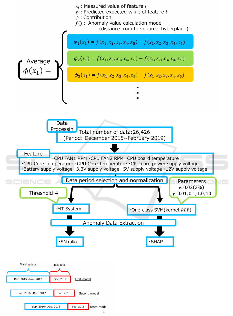
Figure 13: How to calculate contribution in O ne-Class SVM.

Figure 14: Experimental Procedures.

Figure 15: Veriﬁcation Method.

SVM is capable of detecting an omalies at defective

part and detecting signs of anomalies before and after

the defective part. Next, we discuss the results of the

MT method. As shown in Figure a, the MT metho d

can detect anomalies in defective part, but it is n ot as

good as 1-Class SVM in detecting signs of anomalies.

Therefore, we c hecked to see if th e MT method could

predict anomalies by changing the threshold value of

the MT method. The Figure 22 shows time on the

horizontal axis, threshold 4 in red, threshold 3 in light

ICPRAM 2023 - 12th International Conference on Pattern Recognition Applications and Methods

656

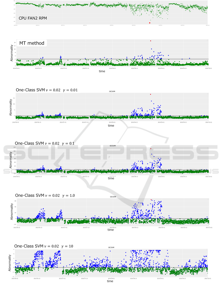
Figure 16: Time series graph of CPU FAN2 RPM. Red dot is 4:00 AM Japan time on August 25, 2018.

Figure 17: Anomaly Graph (MT method).

Figure 18: Anomaly Graph (OCSVM ν = 0.02,γ = 0.01).

Figure 19: Anomaly Graph (OCSVM ν = 0.02,γ = 0.1).

Figure 20: Anomaly Graph (OCSVM ν = 0.02,γ = 1.0).

Figure 21: Anomaly Graph (OCSVM ν = 0.02,γ = 10).

Outlier Detection Method for Equipment Onboard Merchant Vessels

657

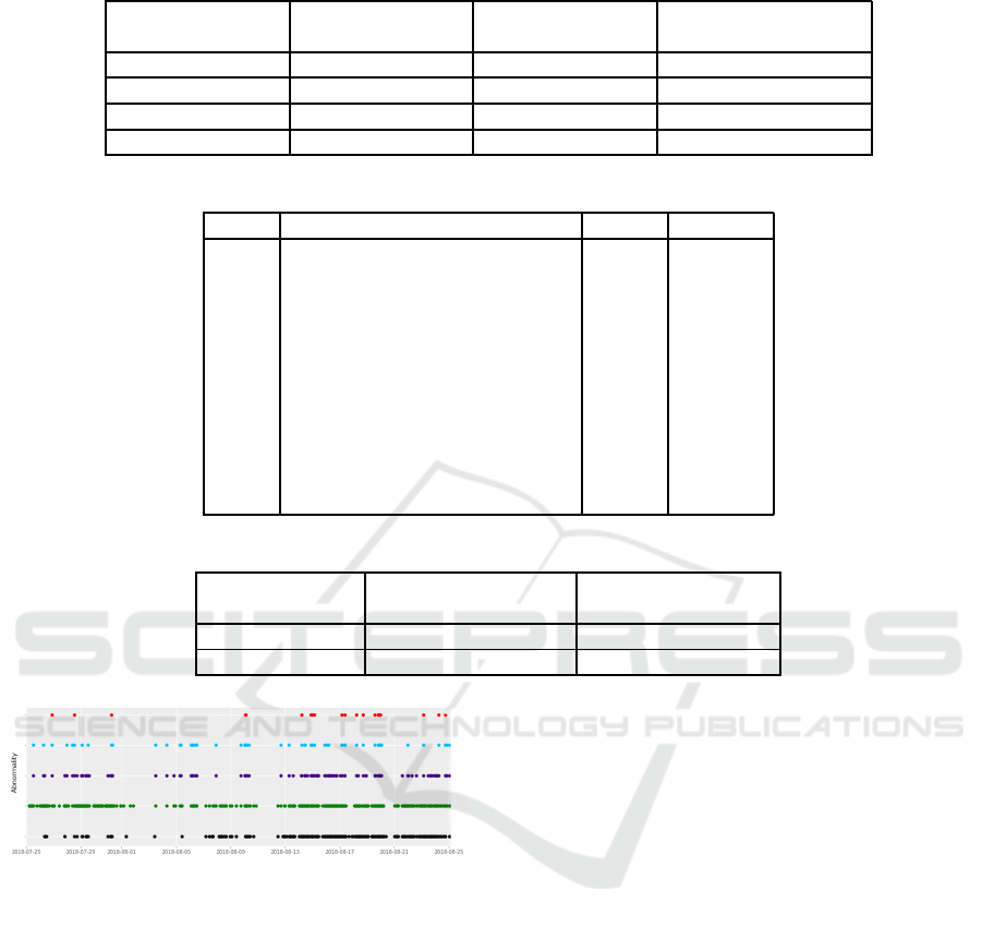
Table 2: Number of anomalies within the set range.

Within one month Within one month Except for one month

Parameters before the defe ct after the defect before and afte r

ν = 0.02 , γ = 0.01 0 1 0

ν = 0.02 , γ = 0.1 0 2 0

ν = 0.02 , γ = 1.0 18 35 0

ν = 0.02 , γ = 10 75 61 177

Table 3: Results of interpretation.

Order Sensor I te m SHAP S/N ratio

1 CPU FAN RPM 0.0056 -5.2943

2 CPU FAN1 RPM 0.0022 -5.90 90

3 CPU FAN2 RPM 1.5895 24.8710

4 CPU board temperature 0.0130 -2.4760

5 CPU Core Tempe rature 0.0 073 -0.7549

6 GPU Core Temperatu re 0.0033 -3.8500

7 CPU core power supply voltage 0.0409 6.4065

8 Battery supply voltage 0.1265 -1.751 6

9 3.3V supply voltage 0.0195 -14.6852

10 5V supply voltage 0.0697 -3.303 1

11 12V su pply voltage 0.1258 -1.4185

Table 4: Results of interpretation

Number of

anomaly detection

Number of

CPU FAN2 RPM

S/N ra tios 23 16

One-Class SVM 204 198

Figure 22: Difference by Threshold.

blue, threshold 2 in purple, thresh old 1 in green, and

One-Class SVM in black. Plotted locations are those

where anomalies are detected . As a precondition, the

detection must be contin uous in order to be reco g-

nized as a pred ictive sign of anomaly. Considering

this, the threshold value m ust be set to 1 in order to

detect signs of anomaly using the MT method. How-

ever, if the threshold is set to 1, 30% of the total data

will be detected as anomaly. This is inappropria te

for an anomaly detection mod el. From the above, we

conclud e that it is difﬁcult for the MT method to de-

tect signs of anomaly in th e present data. On the other

hand, the One- Class SVM was continuously detected

as an anomaly, indicating that it may be effective as

a model for detecting predictive signs of anomalies

approximately one month in advance.

6.3 Contribution Estimation

Experimental Results

Next, we applied the S/N ratios for the MT method

and the SHAP for the One-Class SVM to the defec-

tive part (Table 4). First of all, le t me explain how

to look at Table 4. As for the S/N ratios, a s men-

tioned ea rlier, larger values contribute to that result.

On the other h and, w ith respect to the SHAP values,

they are essentially both positive and negative. This

positive or negative value can measure whether the

data is inﬂuenced by a small or large value. However,

in the ﬁeld of anoma ly detec tion, the most important

question is whether the anomaly is inﬂuenced by, or

could be the cause of, the anomaly. Therefor e, in this

study, SHAP values were converted to absolute values

to make it easier to understand which sensor is inﬂu-

encing. The results of applying the S/N ratios and

SHAP both showed that CPU FAN2 RPM took the

highest value, consistent with the experts that CPU

FAN2 RPM was the cau se of the anomaly. This indi-

cates that both the MT method and One-Class SVM

are suitable for the defective part. Next, we check

the results of the application for data before 4:00 a.m.

on August 25, 2018: anomaly detections for the last

ICPRAM 2023 - 12th International Conference on Pattern Recognition Applications and Methods

658

month as of 4:00 a.m . on A ugust 25, 2018 are shown

in Table 4. Number of anomaly detection in Table 4

indicates the number of times anomaly was detected

out of a total of 723 cases from July 25, 2018 to Au-

gust 25, 2018. The Number of CPU FAN2 RPM indi-

cates the number of times that CPU FAN2 RPM con-

tributed the most out of the Number of anomaly detec-

tions. From the above, it was fou nd that the cause of

the signs o f anomaly is almost the same as the cause

of the defective area in both the MT and One-Class

SVM methods. In particular, One-Class SVM is able

to detec t continuously, making it possible to take ac-

tion o ne month before the expert’s decision.

7 CONCLUSIONS

The equipment onboard merchant vessels are essen-

tial f or safe navigation. However, these devices can-

not be repaired or replaced with the same speed and

accuracy as wh en on land. Ther efore, it is necessary

to detect the signs of an omalies and act with a margin

of error. This paper examines the feasibility of using

the MT method and One-Class SVM to detect signs

of ano malies in equipment on board merchant vessels.

It was shown that both methods can detect the points

pointed out by the person in charge of the equipment.

In addition, One-Class SVM was able to continuously

detect anomalies before the point pointed out by the

person in ch a rge of the model, indicating the possi-

bility of detecting predictive signs of anomalies. In

addition, by ap plying SHAP to One-Class SVM, it be-

came possible to calculate the inﬂuence of each sen-

sor and to identify which senso r value was the cause

of the anomalies. In summary, the proposed method

has the potential to be useful in the maintenance of

equipment onboard merchant vessels.

There are two major issues to be addressed in the

future works. First, the results of this stud y are lim-

ited to a single individual. Th is is partly due to the

fact that, at this point in time, there is still a paucity

of data with records of defects. This is a future issue,

including data collection. The second is the applica-

tion of SHAP to other meth ods. In this study, SHAP

was applied only to th e RBF kernel of the One-Class

SVM. In the future, we will apply SHAP to other out-

lier detection methods to establish the usefulness of

this study.

ACKNOWLEDGEMENTS

This work was partially supported by JST, CREST

(JPMJCR21D4), Japan. We also thank Mr.Hash imoto

who works at Furuno Electric Co. for providing the

data and Mr. Moritoki who works at Lincrea Corpo-

ration for his cooperation in the data analysis.

REFERENCES

Adadi, A. and Berrada, M. (2018). Peeking inside the

black-box: a survey on explainable artiﬁcial intelli-

gence (xai). In IEEE access. IEEE.

Brandsæter, A., Vanem, E., and Glad, I. K. (2019). Efﬁcient

on-line anomaly detection for ship systems in opera-

tion. In Expert Systems with Applications.

Cipollini, F., Oneto, L., Coraddu, A., Murphy, A. J., and

Anguita, D. (2018a). Condition-based maintenance of

naval propulsion systems: Data analysis with minimal

feedback. In Reli ability Engineering & System Safety.

Elsevier.

Cipollini, F., Oneto, L., Coraddu, A., Murphy, A. J., and

Anguita, D. (2018b). C ondition-based maintenance of

naval propulsion systems with supervised data analy-

sis. In Ocean Engineering. Elsevier.

Coraddu, A., Oneto, L., Ghio, A., Savio, S., Anguita, D.,

and Figari, M. (2016). Machine learning approaches

for improving condition-based maintenance of naval

propulsion plants. In Proceedings of the Institution of

Mechanical Engineers, Part M: Journal of Engineer-

ing for the Maritime Environment. SAGE Publications

Sage UK: London, England.

Gunning, D., Steﬁk, M., Choi, J., Miller, T., Stumpf, S., and

Yang, G.-Z. (2019). Xai- explainable artiﬁcial intelli-

gence. In Science robotics. American Association for

the Advancement of Science.

Hotelling, H. (1947). Multivariat e quality control. In Tech-

niques of statistical analysis. McGraw-Hill.

Khan, S. S. and Madden, M. G. (2010). A survey of recent

trends in one class classiﬁcation. In Artiﬁcial Intelli-

gence and Cognitive Science. Springer Berlin Heidel-

berg.

Lazakis, I., Gkerekos, C., and Theotokatos, G. (2019). In-

vestigating an svm-driven, one-class approach to esti-

mating ship systems condition. In Ships and Offshore

Structures. Taylor & Francis.

Lundberg, S. M. and Lee, S.-I. (2017). A uniﬁed approach

to interpreting model predictions. Advances in neural

information processing systems.

Mangalathu, S., Heo, G., and Jeon, J.-S. (2018). Artiﬁcial

neural network based multi - dimensional fragility de-

velopment of skewed concrete bridge classes. In En-

gineering Structures. Elsevier.

Mangalathu, S., Hwang, S.-H., and Jeon, J.-S. (2020). Fail-

ure mode and effects analysis of rc members based on

machine-learning-based shapley additive explanations

(shap) approach. In Engineering Structures. Elsevier.

Porteiro, J., Collazo, J., Pati˜no, D., and M´ıguez, J. L.

(2011). Diesel engine condition monitoring using

a multi-net neural network system with nonintrusive

sensors. In Applied Thermal Engineering. El sevier.

Outlier Detection Method for Equipment Onboard Merchant Vessels

659

Sch¨olkopf, B., Smola, A. J., Williamson, R. C., and Bartlett,

P. L. ( 2000). New support vector algorithms. In Neu-

ral computation. MIT Press One Rogers Street, Cam-

bridge, MA 02142-1209, USA journals-info . . . .

Taguchi, G. and Jugulum, R. (2002). The Mahalanobis-

Taguchi strategy: A pattern technology system. John

Wiley & Sons.

Tan, Y., Tian, H., Jiang, R., Lin, Y., and Zhang, J. (2020). A

comparative investigation of data-driven approaches

based on one-class classiﬁers for condition monitoring

of marine machinery system. In Ocean Engineering.

Elsevier.

Vapnik, V. (1999). The nature of statistical learning theory.

Springer science & business media.

ICPRAM 2023 - 12th International Conference on Pattern Recognition Applications and Methods

660