LSTM, ConvLSTM, MDN-RNN and GridLSTM Memory-based

Deep Reinforcement Learning

Fernando Fradique Duarte

, Nuno Lau

, Artur Pereira

and Luís Paulo Reis

Institute of Electronics and Informatics Engineering of Aveiro, University of Aveiro, Aveiro, Portugal

Department of Electronics, Telecommunications and Informatics, University of Aveiro, Aveiro, Portugal

Faculty of Engineering, Department of Informatics Engineering, University of Porto, Porto, Portugal

Keywords: Convolutional Long Short-Term Memory, Grid Long-Short Term Memory, Long Short-Term Memory,

Mixture Density Network, Reinforcement Learning.

Abstract: Memory-based Deep Reinforcement Learning has been shown to be a viable solution to successfully learn

control policies directly from high-dimensional sensory data in complex vision-based control tasks. At the

core of this success lies the Long Short-Term Memory or LSTM, a well-known type of Recurrent Neural

Network. More recent developments have introduced the ConvLSTM, a convolutional variant of the LSTM

and the MDN-RNN, a Mixture Density Network combined with an LSTM, as memory modules in the context

of Deep Reinforcement Learning. The defining characteristic of the ConvLSTM is its ability to preserve

spatial information, which may prove to be a crucial factor when dealing with vision-based control tasks while

the MDN-RNN can act as a predictive memory eschewing the need to explicitly plan ahead. Also of interest

to this work is the GridLSTM, a network of LSTM cells arranged in a multidimensional grid. The objective

of this paper is therefore to perform a comparative study of several memory modules, based on the LSTM,

ConvLSTM, MDN-RNN and GridLSTM in the scope of Deep Reinforcement Learning, and more specifically

as the memory modules of the agent. All experiments were validated using the Atari 2600 videogame

benchmark.

1 INTRODUCTION

Memory-based Deep Reinforcement Learning has

been shown to be a viable solution to successfully

learn control policies directly from high-dimensional

sensory data in complex vision-based control tasks

such as videogames (Hausknecht & Stone, 2015;

Heess et al., 2015; Sorokin et al., 2015; Tang et al.,

2020). At the core of this success lies the Long Short-

Term Memory (LSTM) (Hochreiter & Schmidhuber,

1997), a very popular Recurrent Neural Network

(RNN), featuring a specialized architecture designed

to overcome the error backflow problems present in

other RNN designs.

Recent developments have introduced the

Convolutional LSTM (ConvLSTM) (Shi et al., 2015),

a convolutional variant of the LSTM, and the Mixture

https://orcid.org/0000-0002-9503-9084

https://orcid.org/0000-0003-0513-158X

https://orcid.org/0000-0002-7099-1247

https://orcid.org/0000-0002-4709-1718

Density Network (MDN) (Bishop, 1994) combined

with an LSTM (MDN-RNN) (Ha & Schmidhuber,

2018) as memory modules in the context of Deep

Reinforcement Learning (DRL). See (Mott et al.,

2019) and (Ha & Schmidhuber, 2018) for examples

of such work.

The defining characteristic of the ConvLSTM is

its ability to preserve spatial information, which may

prove to be a crucial factor when dealing with vision-

based control tasks. The MDN-RNN on the other

hand can be used as a predictive memory (i.e., to

derive a probability distribution of the future),

endowing the agent with the ability to act

instinctively on these predictions of the future without

the need to explicitly plan ahead.

Also of interest to this work is the GridLSTM

(Kalchbrenner et al., 2016), a network of LSTM cells

Duarte, F., Lau, N., Pereira, A. and Reis, L.

LSTM, ConvLSTM, MDN-RNN and GridLSTM Memory-based Deep Reinforcement Learning.

DOI: 10.5220/0011664900003393

In Proceedings of the 15th International Conference on Agents and Artiﬁcial Intelligence (ICAART 2023) - Volume 2, pages 169-179

ISBN: 978-989-758-623-1; ISSN: 2184-433X

 2023 by SCITEPRESS – Science and Technology Publications, Lda. Under CC license (CC BY-NC-ND 4.0)

169

arranged in a multidimensional grid which aims to

further generalize the advantages of LSTMs to the

realm of Deep Neural Networks (DNNs). The focus

of this work is therefore to perform a comparative

study of several memory modules in the context of

DRL and more specifically as the memory modules

of the agent. The four memory modules tested are

based on the LSTM, the ConvLSTM, the MDN-RNN

and the GridLSTM. More concretely, this work aims

to answer the following questions:

 Q1: Can the learning process be improved by

preserving the spatial information inside the

memory module of the agent, when solving

vision-based control tasks directly from high-

dimensional sensory data (e.g., raw pixels)?

 Q2: What are the advantages or disadvantages

of using a contextual memory (e.g., LSTM) as

opposed to a predictive one (e.g., MDN-RNN)?

 Q3: Do different memory modules play

significantly different roles concerning the

decision making of the trained agent?

 Q4: Can the learning process be improved by

using separate memory sub-modules in parallel

(e.g., GridLSTM) to process different

information?

The visualization technique proposed in

(Greydanus et al., 2018) was used to derive further

insight about the different policies learned by the

different memory modules tested. Also, it should be

noted that this work does not address external

memory-based DRL such as in (Graves et al., 2014)

and (Wayne et al., 2018). Finally, the Atari 2600

videogame benchmark was the testbed used to

validate all the experiments. The remainder of the

paper is structured as follows: section 2 presents the

related work, including a brief overview of the

technical background, section 3 discusses the

experimental setup, which includes the presentation

of the methods proposed and the training setup,

section 4 presents the experiments carried out and

discusses the results obtained and finally section 5

presents the conclusions.

2 RELATED WORK

This section presents a brief overview of the related

work and technical background pertinent to this work.

2.1 Memory-based DRL

Many control problems must be solved in partially

observable environments. Most videogames fall into

this category. In the context of Reinforcement

Learning (RL), partial observability means that the

full state of the environment cannot be entirely

observed by an external sensor (e.g., the agent playing

the game). The problem of partial observability arises

frequently in vision-based control tasks, due to for

example, occlusions or the lack of proper information

about the velocities of objects (Heess et al., 2015).

One possible way to address this issue is to

maintain a ‘sufficient’ history of past observations,

which completely describes the current state of the

environment. Deep Q-Network (DQN) (Mnih et al.,

2015) used the last k=4 past observations. The main

drawback of this technique is its heavy reliance on the

value of k, which is task dependent and may be

difficult to derive (Hausknecht & Stone, 2015).

Another possibility is to use RNNs (e.g., LSTM), to

compress this ‘sufficient’ history.

RNNs are well suited to work with sequences and

can act as a form of memory of past observations. The

advantages of this solution are twofold. On one hand

k is no longer necessary, since now the agent only

needs access to the current state of the environment at

each time step t. On the other hand, the agent can now

dynamically learn and determine what a ‘sufficient’

history is accordingly to the needs of the task, which

may entail for example, keeping a compressed history

spanning more than k past observations. Examples of

this work include (Hausknecht & Stone, 2015; Heess

et al., 2015; Sorokin et al., 2015; Tang et al., 2020).

2.2 LSTM and Convolutional LSTM

The LSTM (Hochreiter & Schmidhuber, 1997) was

introduced to solve the error backflow problems

present in other RNN designs. Before the introduction

of the LSTM, RNNs were very unstable and hard to

train, particularly when dealing with longer

sequences (the error signals would either vanish or

blow-up during the optimization process). Since its

introduction the LSTM has gained widespread

popularity in many domains of application such as

speech recognition (Graves et al., 2013), machine

translation (Sutskever et al., 2014) and video

sequence representation (Srivastava et al., 2015).

Equation (1) below, presents the formulation of

the LSTM as implemented in Pytorch (Paszke et al.,

2019), where x

, h

and c

are the input, hidden state

and the cell state at time t, respectively (h

t-1

is the

hidden state at time t-1) and i

, f

and o

are the input,

forget and output gates. W* are the weights and b* the

biases, σ is the sigmoid function and ⊗ represents the

Hadamard product.

ICAART 2023 - 15th International Conference on Agents and Artiﬁcial Intelligence

170

= σ(W

+ b

+ W

-1

+ b

)

(1)

= σ(W

+ b

+ W

-1

+ b

)

= tanh(W

+ b

+ W

-1

+ b

)

= σ(W

+ b

+ W

-1

+ b

)

⊗ c

-1

+ i

⊗

= o

⊗ tanh(c

)

However, LSTMs do not preserve spatial

information, which may be important in vision-based

tasks. The ConvLSTM (Shi et al., 2015) was

proposed to address this issue. The original

formulation of the ConvLSTM follows the one

proposed in the Peephole LSTM (Graves, 2013)

variant and is presented below in Equation (2).

It should be noted however, that in the case of the

ConvLSTM all the involved tensors are 3D, namely,

the x

inputs, the h

hidden states, the c

cell states and

the i

, f

and o

gates. An example of this work can be

found in (Mott et al., 2019) where the authors used a

ConvLSTM in their vision core to implement an

attention-augmented RL agent.

= σ(W

+ W

-1

+ W

⊗ c

-1

+ b

)

= σ(W

+ W

-1

+ W

⊗ c

-1

+ b

)

⊗ c

-1

+ i

⊗tanh(W

+ W

-1

+ b

)

(2)

= σ(W

+ W

-1

+ W

⊗ c

+ b

)

⊗ tanh(c

)

2.3 GridLSTM

Similarly to RNNs, DNNs can suffer from the

vanishing gradient problem when applied to longer

sequences. Also, in a DNN, layers have no inbuilt

mechanisms to dynamically select or ignore parts or

the whole of their inputs. The GridLSTM

(Kalchbrenner et al., 2016) was proposed to address

these issues, further generalizing the advantages of

LSTMs to the realm of DNNs.

At a high level, a GridLSTM is a neural network

that is arranged in a grid with one or more

dimensions. Layers communicate with each other

directly through LSTM cells which can be placed

along any (or all) of these dimensions. Among other

things, the GridLSTM also proposes an efficient N-

way communication mechanism across the LSTM

cells, allows dimensions to be prioritized as well as

non-LSTM dimensions and promotes more compact

models by allowing the weights to be shared among

all the dimensions (referred to as a Tied N-LSTM).

2.4 MDN-RNN

The MDN (Bishop, 1994) combines a neural network

with a mixture density model and can in principle

represent arbitrary conditional probability

distributions. More formally, given an output y and an

input x, and modeling the generator of the data y

∈

as a mixture model (e.g., Gaussian Mixture Model),

the probability density of the target data can be

represented as in Equation (3) below. The parameters

(x), referred to as the mixing components, can be

regarded as prior probabilities (i.e., each α

(x)

represents the prior probability of the target y having

been generated from the ith component of the

mixture) and the functions ϕ

(y|x) represent the

conditional density of the target y for the ith kernel.

𝑝



𝑦

𝑥) = 𝛼





𝑥

)

𝜙





𝑦

𝑥)







)

The work in (Ha & Schmidhuber, 2018) combined

an MDN with an LSTM, referred to as MDN-RNN,

to derive a predictive memory of the future

P(z

t+1

, a

, h

), where z

, a

and h

are the latent vector

encoded by the convolutional network, the action

performed and the hidden state of the RNN at time

step t respectively, which the agent can query in order

to act without the need to plan ahead.

The present work leverages all of the work

presented in this section to perform a comparative

study over all these techniques in the context of

memory-based DRL.

3 EXPERIMENTAL SETUP

This section presents the experimental setup used,

including the presentation of the memory modules

proposed and the training setup.

3.1 Baseline Agent

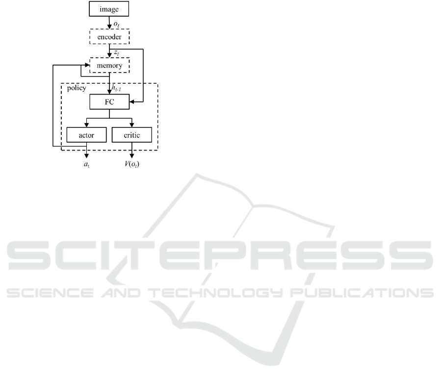
At a high level, the baseline architecture used to

compose the agents comprises three main modules,

namely: the encoder, the memory and the policy. At

each time step t, the encoder receives a single image

, representing the current state of the game and

encodes it into a set of feature maps z

. Based on z

and the hidden state of the memory module at the

previous time step h

t-1

, the policy chooses an action a

and acts on the environment. Finally, z

, a

and h

t-1

are

passed to the memory module, which in turn

computes the next hidden state h

, see Figure 1.

While this architecture is common to all the agents

tested, the internal details of the memory module

differ and shall be addressed when appropriate. As for

the encoder, the only difference is that all the LSTM-

LSTM, ConvLSTM, MDN-RNN and GridLSTM Memory-based Deep Reinforcement Learning

171

based agents use l=5 convolutional layers whereas all

the ConvLSTM-based agents use only l=4. In both

cases the encoders are configured in a similar way.

The policy module is common to all the agents.

Figure 1: Baseline architecture of the agents, depicting the

information flow. The three main modules, encoder,

memory and policy are highlighted in dashed boxes.

More concretely, and regarding the baseline

agent, referred henceforth as LSTM, the encoder is

composed of l=5 convolutional layers configured

with (1, 32, 64, 64, 64) input channels, (32, 64, 64,

64, 64) output channels, kernel sizes (8, 4, 4, 4, 4),

strides (4, 2, 2, 1, 1) and no padding, respectively.

Each layer is followed by batch normalization (Ioffe

& Szegedy, 2015) and a Rectified Linear Unit

(ReLU) nonlinearity. The memory module in turn is

composed by an LSTM with size 256 (the Pytorch

implementation was used).

Finally, the policy comprises a linear layer

(denoted as FC in the figure) with size 128 followed

by layer normalization (Ba et al., 2016) and a ReLU

nonlinearity, which feeds into two other linear layers,

the actor and the critic, responsible for choosing the

actions and computing the value of the state,

respectively.

3.2 ConvLSTM-based Agent

The encoder used by this agent, referred to as

ConvLSTM, uses l=4 convolutional layers. The

reasons to use l=4 as opposed to l=5 are twofold: 1)

some quick empirical tests seemed to indicate that the

ConvLSTM performed better with l=4 and 2) using

l=4 allowed the number of parameters of both the

LSTM and the ConvLSTM-based agents to be almost

identical (with the exception of the MDN-RNN case),

thus excluding this (i.e., the number of parameters) as

a possible explanatory factor when comparing the

agents performance wise.

Finally, the memory module comprises a

ConvLSTM with size 64x8x5 (i.e., a volume with 64

channels of height 8 and width 5). The

implementation used is similar to Equation (1), the

main differences being that: 1) all the inputs, outputs

and gates are 3D and 2) x

and h

t-1

are concatenated,

not added together. It should be noted that in all the

agents tested, except the 2-GridLSTM agent,

= (z

, a

), that is, x

is derived by concatenating z

and a

. Also note that Equation (1) was used in favour

of Equation (2) mainly due to its greater simplicity.

As a final note, both the MDN-RNN and the

GridLSTM-based memory modules, presented next,

were implemented using the ConvLSTM. The two

main reasons for this were: 1) the ConvLSTM has

been less explored in the literature when compared to

the LSTM and 2) because the ConvLSTM preserves

spatial information, which may allow visualization

techniques such as the one proposed in (Greydanus et

al., 2018) to be used to try to get better insights

regarding the role of memory in the decision making

of the trained agent. However, in the case of the

GridLSTM, yet a different approach uses both an

LSTM and a ConvLSTM in parallel.

3.3 MDN-RNN-based Agent

This agent, henceforth referred to as MDN-RNN, uses

an l=4 encoder, for the reasons already mentioned.

Also, similarly to the ConvLSTM agent, the memory

module comprises a ConvLSTM with size 64.

Excluding the fact that the memory module is based

on the ConvLSTM, the implementation of the MDN-

RNN follows the one proposed in (Ha &

Schmidhuber, 2018) and (Bishop, 1994).

3.4 GridLSTM-based Agents

Two different memory modules were tested in this

category. The memory module of the first agent,

referred to as GridLSTM, was composed by adapting

the implementation of the GridLSTM to work with a

vanilla ConvLSTM, similar to the one used in the

ConvLSTM agent. The memory module of the second

agent implemented, referred to as 2-GridLSTM, on

the other hand, exploits the fact that different

information is being passed to memory.

As already mentioned and depicted in Figure 1

and also of interest to the following discussion, the

memory module receives z

and a

as inputs at each

time step t. On top of representing two different

pieces of information, the format of these two inputs

ICAART 2023 - 15th International Conference on Agents and Artiﬁcial Intelligence

172

is also different (3D and 1D respectively). This in turn

opens the opportunity to process each piece of

information separately (and in parallel) using a

memory sub-module suited to their format. This is the

purpose of the 2-GridLSTM agent.

Contrary to all other agents, where z

is flattened

and concatenated with a

, the memory module of the

2-GridLSTM agent processes z

and a

separately and

in parallel using a ConvLSTM (size 64) and an LSTM

(size 64) respectively. In Figure 1, h

t-1

= (h

t-1

where the first memory component h

t-1

corresponds

to the hidden state of the ConvLSTM and the second

memory component h

t-1

corresponds to the hidden

state of the LSTM. The ConvLSTM preserves the

spatial information contained in z

whereas a

(one-hot

encoded in this case) can be processed by an LSTM

since it does not hold any spatial information. More

specifically, this flow of information occurs over the

depth dimension.

As a final note, the GridLSTM agent uses shared

weights across dimensions. Also, the depth

dimension is prioritized in both agents. Finally, both

agents use an l=4 encoder similar to the one used by

the ConvLSTM agent.

3.5 Training Setup

In terms of pre-processing steps, the input image at

each time step t is converted to grayscale and cropped

to 206 by 158 pixels to better fit the encoder used. No

rescaling is performed. All agents are trained for a

minimum of 16,800,000 frames, which can be

extended until all current episodes are concluded,

similarly to what is proposed in (Machado et al.,

2018). In this context an episode is a set of m lives.

A total of eight training environments were used

in parallel to train the agent using the Advantage

Actor-Critic (A2C) algorithm, a synchronous version

of the Asynchronous Advantage Actor-Critic (A3C)

(Mnih et al., 2016). Adam (Kingma & Ba, 2015) was

used as the optimizer. The learning rate is fixed and

set to 1e-4. The loss was computed using Generalized

Advantage Estimation with λ=1.0 (Schulman et al.,

2016).

In terms of the remaining hyperparameters used,

an entropy factor was added to the policy loss with a

scaling factor of 1e-2, the critic loss was also scaled

by a factor of 0.5, rewards were clipped in the range

[-1, 1] and a discount factor of γ=.99 was used. No

gradient clipping was performed. Concerning frame

skipping, this is in-built in OpenAI Gym (Brockman

et al., 2016) (i.e., at each step t OpenAI Gym will skip

between two to four frames randomly).

Finally, at the beginning of training the internal

state of the memory component is set to an empty

state (i.e., all zeros) representing the state of no

previous knowledge. and is never reset to zero during

the remainder of the training procedure (e.g., at the

end of each episode or life).

It should also be noted that during training (i.e.,

backpropagation) the gradient flow from the memory

module to the encoder is cut. This is done to ensure

that the memory module only manages information as

opposed to also participate in its optimization. This

compartmentalization allows the scrutiny of the

responsibility of the memory module as a standalone

factor concerning the decision making of the trained

agent. The number of trainable parameters for each of

the memory modules implemented is as follows:

LSTM 1,287,795, ConvLSTM 1,161,395, MDN-RNN

5,109,181, GridLSTM 1,276,787 and 2-GridLSTM

1,424,243.

4 EXPERIMENTAL RESULTS

This section presents the training and test results

obtained. Each different memory module

implemented was trained using three agents

initialized with different seeds The training results

were computed at every 240,000

frame over a

window of size w=50 and correspond to the return

scores (averaged over all the agents) obtained during

training in the last w fully completed episodes. After

the training process was completed, each of the three

agents trained, played 100 games for a total of 300

games which were used to derive the test results. For

the statistical significance tests both the one-way

ANOVA as well as the Kruskal-Wallis H-test for

independent samples were used with α=0.05.

The benchmark used to perform and validate the

experiments was the Atari 2600 videogame platform,

available via the OpenAI Gym toolkit. Due to

hardware and time constraints only two games were

used, namely, RiverRaid and ChopperCommand.

These games were selected given that their

performance, as presented in (Mnih et al., 2015), was

below human level (57.3% and 64.8% respectively),

but not so low that it prevented the agents from

learning any meaningful policy. These games also

present a wide range of different challenges. In

RiverRaid the agent must manoeuvre over sometimes

narrow waterways while avoiding the enemies trying

to intercept and destroy it and refuelling to avoid

death. In ChopperCommand the agent must destroy

the enemy airships while avoiding their projectiles.

LSTM, ConvLSTM, MDN-RNN and GridLSTM Memory-based Deep Reinforcement Learning

173

4.1 Results

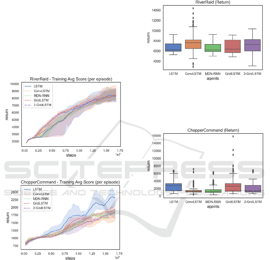
Figures 2 and 3 below, present the training results

obtained for RiverRaid and ChopperCommand,

respectively. As it can be seen, in the case of

Riverraid, all agents seem to exhibit a plateauing

behaviour during the initial phase of training, which

can be more prolonged for some of the agents (e.g.,

LSTM and GridLSTM). At the end of training,

however, all the agents seem to achieve roughly the

same performance. Regarding ChopperCommand,

the LSTM agent seems to learn much more rapidly

than the ConvLSTM-based agents.

Figure 2: Training return per episode for RiverRaid. The

confidence interval used was .95.

Figure 3: Training return per episode for

ChopperCommand. The confidence interval used was .95.

Much more interesting are the return (or

cumulative reward) results obtained by the trained

agents. Performance wise the best agents were the

ConvLSTM agent in Riverraid and the LSTM agent in

ChopperCommand (although followed very closely

by the GridLSTM agent), see Figure 4 and Figure 5,

respectively. These results are also statistically

significant: we reject the null hypothesis (H

) that all

the agents have the same return mean results, with p-

values 2.1e-70 and 6.7e-51 for the ANOVA and 4.6

e-50 and 3.8e-50 for the H-test for RiverRaid and

ChopperCommand, respectively.

Figure 4: Test return per episode for RiverRaid. The overall

median values as well as the average result and standard

deviation obtained by the best agent for each memory

module were: LSTM 6205 (7600/726), ConvLSTM 7605

(8090/2076), MDN-RNN 6160 (7225/765), GridLSTM

6330 (7618/831) and 2-GridLSTM 7265 (7997/1050).

Figure 5: Test return per episode for ChopperCommand.

The results are presented similarly to Figure 4 and were:

LSTM 2700 (3003/948), ConvLSTM 1300 (2302/1285),

MDN-RNN 1200 (2147/1117), GridLSTM 2600

(3814/2362) and 2-GridLSTM 1400 (2447/1242).

Also, the difference observed in the return results

obtained by the LSTM and MDN-RNN agents in

RiverRaid does not seem to hold statistical

significance (H

is not rejected with p-values 0.13 for

the ANOVA and 0.07 for the H-test). Similarly, in

ChopperCommand the difference observed in the

return results obtained by the ConvLSTM and MDN-

RNN agents and the LSTM and GridLSTM agents

does not seem to hold statistical significance: in the

first case H

is not rejected with p-values 0.4 for the

ANOVA and 0.1 for the H-test and in the second case

is not rejected with p-values 0.7 for the ANOVA

and 0.08 for the H-test.

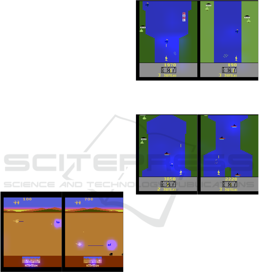
These tests were also performed using an image

perturbed with gaussian noise with σ=.1, see Figure

ICAART 2023 - 15th International Conference on Agents and Artiﬁcial Intelligence

174

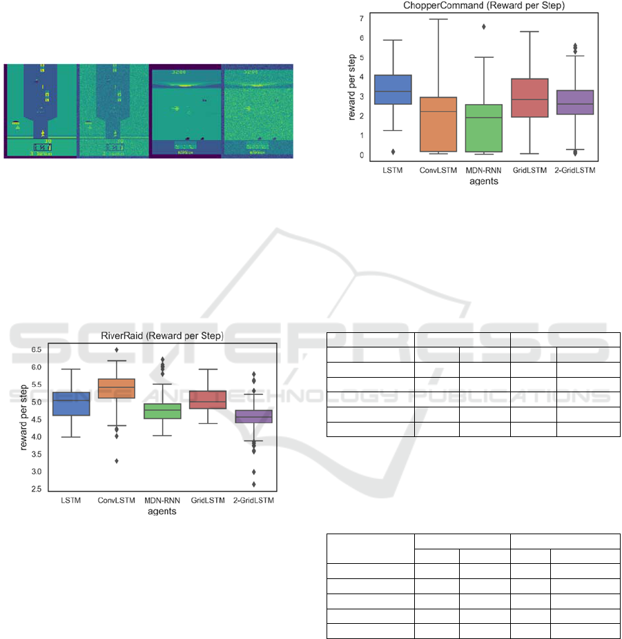
6. The percentage reduction ratios for each agent were

the following (for RiverRaid and ChopperCommand

respectively): LSTM (57/59)%, ConvLSTM (29/38)%,

MDN-RNN (55/50)%, GridLSTM (20/65)% and 2-

GridLSTM (59/21)%. As it can be seen by the results,

and overall, the ConvLSTM agent seemed to be more

resilient to the noise introduced to the image. The

remaining agents suffered a loss in performance

greater or equal than 50% in one or both games.

Figure 6: Examples of image perturbation for Riverraid

(second image) and ChopperCommand (last image).

To try to assess possible behavioural differences

in the different memory modules, the results for the

‘number of steps’ and ‘reward per step’ obtained

during testing were also investigated, see Figure 7 and

Figure 8 for a graphical depiction of the results for the

latter and consult Table 1 and Table 2 for the

numerical results concerning both experiments.

Figure 7: Test reward obtained per step (per episode) for

RiverRaid.

After inspection, it can be seen that, similarly to

the results obtained for the return experiments, the

agents with the highest reward/step ratio are the

ConvLSTM agent for RiverRaid and the LSTM agent

in the case of ChopperCommand. An interesting note

to point out, concerning the results in Riverraid, is the

fact that although being the second-best performant

agent in this game, the 2-GridLSTM agent presents

the lowest reward per step among all agents (and also

the highest number of steps, which explains its second

place). Also noteworthy is the low reward/step ratio

of the ConvLSTM and MDN-RNN agents in

ChopperCommand when compared to the high

number of steps achieved by their best agents. After

visual inspection it was found that in certain points of

the game the agent would just turn the chopper

alternately back and forth for a considerable amount

of time.

Figure 8: Test reward obtained per step (per episode) for

ChopperCommand.

Table 1: Test results for the ‘reward per step’ and ‘number

of steps’ experiments in RiverRaid. The overall median

values as well as the average result and standard deviation

obtained by the best agent for each memory module are

depicted. In both cases the differences found on the results

were statistically significant.

RiverRai

reward per step number of steps

Best Me

Best

LSTM 5 5.2/0.3 1339 1445/116

ConvLSTM 5.4 5.6/0.3 1362 1554/340

MDN-RNN 4.8 5/0.3 1328 1507/130

GridLSTM 5 5.2/0.3 1299 1455

123

2- GridLSTM 4.6 4.7/0.3 1568 1688

231

Table 2: Test results for the ‘reward per step’ and ‘number

of steps’ experiments in ChopperCommand. The results are

presented similarly to Table 1. Again, in both cases the

differences found on the results were statistically

significant.

Chopper

Command

reward

er ste

number of ste

Best Me

Best

LSTM 3.3 3.7/1.0 721 967/1852

ConvLSTM 2.2 2.9/1.0 814 7275/4161

MDN-RNN 1.9 2.2/0.9 844 5585/4637

GridLSTM 2.8 3.6/1.0 842 2927

3799

2- GridLSTM 2.6 3.2/1.0 633 2344/3708

The last experiment carried out consisted of

testing the trained agents without their memory

component. In other words, at each time step t, h

t-1

was completely zeroed out before being inputted into

the policy, which means that the only information

available to the trained agent was z

(the latent vector

representing the current screen of the game). This also

means that when analysing the results, the greater the

LSTM, ConvLSTM, MDN-RNN and GridLSTM Memory-based Deep Reinforcement Learning

175

reduction ratio observed in the performance, the more

reliant the agent is on its memory module. If on the

other hand there is no significant change in

performance or performance increases, this may be a

hint that the agent does not rely on its memory

module. This may be the case for example, due to a

poor-quality memory module (obtained after

optimization) or simply because the agent was able to

memorize the dynamics of the game to some extent.

When compared to the results presented in Figure

4 and Figure 5 we see that for RiverRaid the

percentage reduction ratio was: LSTM 2.6%,

ConvLSTM 26.6%, MDN-RNN 0.16% increase,

GridLSTM 19.95% increase and 2-GridLSTM 15.8%.

Interestingly, both the MDN-RNN and the GridLSTM

agents improved their return performance values

when the memory component was removed from the

policy input. The differences observed for the MDN-

RNN agent were however not statistically significant

(p-value 0.58 for the ANOVA and 0.62 for the H-

test). The differences observed for the GridLSTM

agent on the other hand were statistically significant

(p-value 9.8e-6 for the ANOVA and 3.5-e5 for the H-

test). For ChopperCommand, removing the memory

information did not produce any (statistically)

significative changes, except for the GridLSTM agent

with a percentage reduction ratio of 42%.

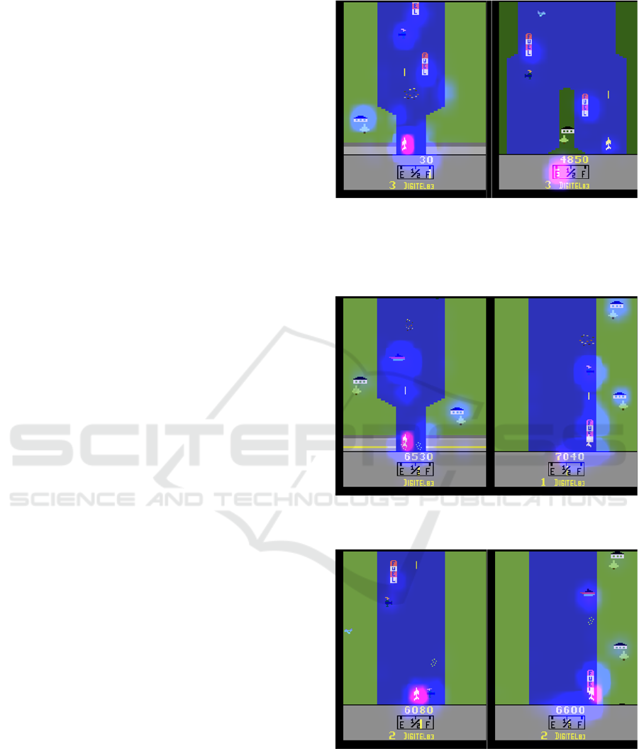
4.2 Saliency Visualization

The saliency metric proposed in (Greydanus et al.,

2018) was used to better assess the different agents

implemented. For this purpose, the saliency maps

were derived using both image perturbation, as

proposed by the referred paper, and memory

perturbation. Memory perturbation was achieved,

similarly to image perturbation, but in this work the

memory positions were zeroed out as opposed to

‘blurred’. Memory perturbation is possible this way

since the ConvLSTM preserves spatial information.

The results reported here were derived by taking

the best trained agent for each memory module,

running it over 20 games and then choosing the game

where the agent achieved a better return score to

perform saliency visualization. The policy network

saliency is displayed in blue whereas the value

network policy is displayed in red. Also, since the

results obtained in ChopperCommand were very poor

for most of the agents, the saliency visualization is

performed mostly in RiverRaid. Figures 9, 10 and 11

depict the saliency maps derived for the memory

agents using image perturbation for Riverraid.

Figure 9: The LSTM agent focusing on the main elements

of the game (left). The value network saliency of the

ConvLSTM agent seems to recognize the value inherent to

having the tank almost empty but still the agent does not

refuel and ends up dying (right).

Figure 10: The MDN-RNN agent focusing on its projectile

(left). The GridLSTM agent refuelling (right).

Figure 11: The 2-GridLSTM agent: near miss (left) and

refuelling for the second time (right).

Generally speaking, all of the agents seem to

focus on the main elements of the game, namely: the

enemies near or further away, the riverbank closer to

the agent and the agent projectile. However, none of

the agents seems to have learned to refuel in a

ICAART 2023 - 15th International Conference on Agents and Artiﬁcial Intelligence

176

consistent way. Some agents seem to focus their value

network on the display information showing that the

tank is empty (e.g., LSTM) but never attempt to refuel,

while others refuel although not in a consistent away

(i.e., GridLSTM one time and 2-GridLSTM two

times).

Overall, the difference in performance observed

seems to stem from how the agents prioritize their

targets and how assertive they are at destroying or

avoiding their enemies and avoiding crashing into the

riverbank. The ConvLSTM agent seems to be better at

this, together with the LSTM agent. The remaining

agents seem to have more trouble choosing their

targets, miss more shoots, seem to be more undecisive

at times, MDN-RNN in particular, gets too close to its

enemies, making it more prone to collisions, and

GridLSTM and 2-GridLSTM are prone to colliding

with the riverbank.

Figure 12 below, depicts the same saliency maps

for ChopperCommand. Overall, all the agents seem to

concentrate on the main elements of the game,

namely: the mini map, the enemies, near or further

away and the agent itself. However, none of the

agents has learned to focus on the projectiles fired by

the enemy fighters. Performance wise both the LSTM

and GridLSTM agents seem to be more assertive and

better at destroying and avoiding the enemy fighters.

The 2-GridLSTM agent for example, often fails to

destroy the enemy fighters and ends up suffering from

frequent near misses due to that fact, which hinders

its performance.

Figure 12: The LSTM agent is focused on the mini map as

well as on its closest enemy (left). Similarly, the GridLSTM

agent is also focused on the same areas and also on the agent

itself (right). None of the agents is focused on the projectiles

fired by the enemy fighters.

Concerning memory perturbation, and generally

speaking, all the memory modules seem to be more

active and focused on the area immediately in front of

the agent and also on the closest enemy. Interestingly,

the area of focus seems to mimic the lateral

movement of the enemies, see Figure 13 and 14.

Figure 13: The memory module of the ConvLSTM agent is

focused on the closest enemy and mimics its lateral

movement (left). The memory activation of the MDN-RNN

agent is faintly focused on the closest enemy (right).

Figure 14: The memory module of the GridLSTM agent is

focused on the closest enemy and mimics its lateral

movement and will focus on the next enemy (left). The

memory activation of the 2- GridLSTM agent is focused on

the closest enemy (just destroyed) and also on a further

away enemy (right).

4.3 Discussion

Concerning Q1 and considering the results obtained

in Riverraid, it seems that at least in some cases

preserving the spatial information does indeed help

improve the quality of the trained agents. Proof of this

is the fact that all ConvLSTM-based agents, with the

exception of the MDN-RNN agent (which obtained

similar results) obtained better performance results

than the LSTM agent. The poor results obtained by the

ConvLSTM-based agents in ChopperCommand,

alongside the better performance obtained by their

GridLSTM-based counterparts, on the other hand,

may be an indication that the ConvLSTM is likely to

be more sensitive to the architecture of the encoder or

LSTM, ConvLSTM, MDN-RNN and GridLSTM Memory-based Deep Reinforcement Learning

177

and memory module or even the size of the memory

itself due to the fact that it is preserving spatial

information.

Regarding Q2, the results do not seem to support

any evidence that a predictive memory such as the

MDN-RNN brings any benefit over the use of a

contextual memory (e.g. LSTM), at least under the

context of the experiments performed. It should be

noted however, that the MDN-RNN relies on the

predictions of a predictive model (being optimized

simultaneously with the agent), which may be wrong

sometimes.

Concerning Q3 and considering Riverraid, it

seems to be the case that in fact different memory

modules produce different behaviours. The

ConvLSTM and LSTM agents seem to be more

greedy, decisive, assertive and efficient whereas

MDN-RNN is prone to near misses and collisions with

the enemies and GridLSTM and 2-GridLSTM are

prone to colliding with the riverbank (and also

enemies to a lesser extent). Some hints to this can be

seen in Table 1, concerning the ‘reward per step’ and

‘number of steps’ results.

Finally, regarding Q4, the results do not seem to

decisively support any claim that using separate

memory sub-modules in parallel brings any

significant improvement in terms of the policies

obtained. While the 2-GridLSTM agent performed

better than the GridLSTM agent in Riverraid, this was

due to a higher number of steps, since the reward per

step obtained was the lowest among all the agents

(and in particular GridLSTM). On the other hand, in

ChopperCommand the GridLSTM agent performed

better than 2-GridLSTM.

5 CONCLUSIONS

Memory-based DRL has achieved much success and

will likely continue to do so. As more memory

architectures and designs are proposed and evolve

over time it is important to perform comparative

studies to assess their capabilities. This was the focus

of this work. For this purpose, four memory modules

based on the LSTM, ConvLSTM, MDN-RNN and

GridLSTM were assessed in the context of DRL,

using the Atari 2600 gaming platform as a testbed.

The results reported here are merely indicative as the

modules used were parameterized out of the box and

further fine tuning, whether be it the architecture of

the encoder and or the memory module or the size of

the memory may significantly improve the results.

ACKNOWLEDGEMENTS

This research was funded by Fundação para a Ciência

e a Tecnologia, grant number SFRH/BD/145723

/2019 - UID/CEC/00127/2019.

REFERENCES

Ba, L. J., Kiros, J. R., & Hinton, G. E. (2016). Layer

Normalization. CoRR, abs/1607.06450. http://

arxiv.org/abs/1607.06450

Bishop, C. M. (1994). Mixture Density Networks.

Brockman, G., Cheung, V., Pettersson, L., Schneider, J.,

Schulman, J., Tang, J., & Zaremba, W. (2016). OpenAI

Gym. CoRR, abs/1606.01540. http://arxiv.org/

abs/1606.01540

Graves, A. (2013). Generating Sequences With Recurrent

Neural Networks. CoRR, abs/1308.0850. http://

arxiv.org/abs/1308.0850

Graves, A., Mohamed, A., & Hinton, G. E. (2013). Speech

recognition with deep recurrent neural networks. IEEE

International Conference on Acoustics, Speech and

Signal Processing, ICASSP 2013, 6645–6649

Graves, A., Wayne, G., & Danihelka, I. (2014). Neural

Turing Machines. CoRR, abs/1410.5401.

http://arxiv.org/abs/1410.5401

Greydanus, S., Koul, A., Dodge, J., & Fern, A. (2018).

Visualizing and Understanding Atari Agents. In

Proceedings of the 35th International Conference on

Machine Learning, ICML 2018, (Vol. 80, pp. 1787–

1796). PMLR

Ha, D., & Schmidhuber, J. (2018). World Models. CoRR,

abs/1803.10122. http://arxiv.org/abs/1803.10122

Hausknecht, M., & Stone, P. (2015). Deep Recurrent Q-

Learning for Partially Observable MDPs. AAAI Fall

Symposium - Technical Report, FS-15-06, 29–37

Heess, N., Hunt, J. J., Lillicrap, T. P., & Silver, D. (2015,

December 14). Memory-based control with recurrent

neural networks

Hochreiter, S., & Schmidhuber, J. (1997). Long Short-Term

Memory. Neural Computation, 9(8), 1735–1780.

Ioffe, S., & Szegedy, C. (2015). Batch Normalization:

Accelerating Deep Network Training by Reducing

Internal Covariate Shift. In Proceedings of the 32nd

International Conference on Machine Learning, ICML

2015, (Vol. 37, pp. 448–456). JMLR.org

Kalchbrenner, N., Danihelka, I., & Graves, A. (2016). Grid

Long Short-Term Memory. In 4th International

Conference on Learning Representations, ICLR 2016

Kingma, D. P., & Ba, J. (2015). Adam: A Method for

Stochastic Optimization. In 3rd International

Conference on Learning Representations, ICLR 2015,

Conference Track Proceedings

Machado, M. C., Bellemare, M. G., Talvitie, E., Veness, J.,

Hausknecht, M. J., & Bowling, M. (2018). Revisiting

the Arcade Learning Environment: Evaluation

ICAART 2023 - 15th International Conference on Agents and Artiﬁcial Intelligence

178

Protocols and Open Problems for General Agents. J.

Artif. Intell. Res., 61, 523–562

Mnih, V., Badia, A. P., Mirza, M., Graves, A., Lillicrap, T.

P., Harley, T., Silver, D., & Kavukcuoglu, K. (2016).

Asynchronous Methods for Deep Reinforcement

Learning. In Proceedings of the 33nd International

Conference on Machine Learning, ICML 2016, (Vol.

48, pp. 1928–1937)

Mnih, V., Kavukcuoglu, K., Silver, D., Rusu, A. A.,

Veness, J., Bellemare, M. G., Graves, A., Riedmiller,

M. A., Fidjeland, A., Ostrovski, G., Petersen, S.,

Beattie, C., Sadik, A., Antonoglou, I., King, H.,

Kumaran, D., Wierstra, D., Legg, S., & Hassabis, D.

(2015). Human-level control through deep

reinforcement learning. Nat., 518(7540), 529–533

Mott, A., Zoran, D., Chrzanowski, M., Wierstra, D., &

Rezende, D. J. (2019). Towards Interpretable

Reinforcement Learning Using Attention Augmented

Agents. In Advances in Neural Information Processing

Systems 32: Annual Conference on Neural Information

Processing Systems 2019, NeurIPS 2019, (pp. 12329–

12338)

Paszke, A., Gross, S., Massa, F., Lerer, A., Bradbury, J.,

Chanan, G., Killeen, T., Lin, Z., Gimelshein, N.,

Antiga, L., Desmaison, A., Köpf, A., Yang, E. Z.,

DeVito, Z., Raison, M., Tejani, A., Chilamkurthy, S.,

Steiner, B., Fang, L., … Chintala, S. (2019). PyTorch:

An Imperative Style, High-Performance Deep Learning

Library. In Advances in Neural Information Processing

Systems 32: Annual Conference on Neural Information

Processing Systems 2019, NeurIPS 2019, (pp. 8024–

8035)

Schulman, J., Moritz, P., Levine, S., Jordan, M. I., &

Abbeel, P. (2016). High-Dimensional Continuous

Control Using Generalized Advantage Estimation. In

4th International Conference on Learning

Representations, ICLR 2016

Shi, X., Chen, Z., Wang, H., Yeung, D.-Y., Wong, W.-K.,

& Woo, W. (2015). Convolutional LSTM Network: A

Machine Learning Approach for Precipitation

Nowcasting. In Advances in Neural Information

Processing Systems 28: Annual Conference on Neural

Information Processing Systems 2015, (pp. 802–810)

Sorokin, I., Seleznev, A., Pavlov, M., Fedorov, A., &

Ignateva, A. (2015). Deep Attention Recurrent Q-

Network. CoRR, abs/1512.01693. http://arxiv.org/

abs/1512.01693

Srivastava, N., Mansimov, E., & Salakhutdinov, R. (2015).

Unsupervised Learning of Video Representations using

LSTMs. In Proceedings of the 32nd International

Conference on Machine Learning, ICML 2015, (Vol.

37, pp. 843–852)

Sutskever, I., Vinyals, O., & Le, Q. v. (2014). Sequence to

Sequence Learning with Neural Networks. In

Advances in Neural Information Processing Systems

27: Annual Conference on Neural Information

Processing Systems 2014, (pp. 3104–3112)

Tang, Y., Nguyen, D., & Ha, D. (2020). Neuroevolution of

self-interpretable agents. In GECCO ’20: Genetic and

Evolutionary Computation Conference, 2020 (pp. 414–

424). ACM.

Wayne, G., Hung, C.-C., Amos, D., Mirza, M., Ahuja, A.,

Grabska-Barwinska, A., Rae, J. W., Mirowski, P.,

Leibo, J. Z., Santoro, A., Gemici, M., Reynolds, M.,

Harley, T., Abramson, J., Mohamed, S., Rezende, D. J.,

Saxton, D., Cain, A., Hillier, C., … Lillicrap, T. P.

(2018). Unsupervised Predictive Memory in a Goal-

Directed Agent. CoRR, abs/1803.10760. http://

arxiv.org/abs/1803.10760.

LSTM, ConvLSTM, MDN-RNN and GridLSTM Memory-based Deep Reinforcement Learning

179