Spectral Analysis of Cardiogenic Vibrations to Distinguish Between

Valvular Heart Diseases

Ecem Erin

and Beren Semiz

2 a

Department of Physics, Bogazici University, Istanbul, Turkey

Department of Electrical and Electronics Engineering, Koc University, Istanbul, Turkey

Keywords:

Seismocardiogram, Cardiovascular Health Monitoring, Valvular Heart Disease, Biomedical Signal Processing.

Abstract:

Cardiovascular diseases are one of the top causes of mortality, accounting for a sizeable portion of all fatalities

globally. Among cardiovascular diseases, valvular heart diseases (VHDs) affect greater number of people

and have higher mortality rates. Current VHD assessment methods are cost-inefﬁcient and limited to clinical

settings, therefore there is a compelling need for non-invasive and continuous VHD monitoring systems. In this

work, a novel framework was proposed to distinguish between aortic stenosis (AS), aortic valve regurgitation

(AR), mitral valve stenosis (MS), and mitral valve regurgitation (MR) using tri-axial seismocardiogram (SCG)

signals acquired from the mid-sternum. First, seismology domain knowledge was leveraged and applied to

SCG signals through ObsPy toolbox for pre-processing. From pre-processed signal segments, spectrogram,

wavelet, chromagram, tempogram and zero-crossing-rate features were extracted. Following p-value analysis

and variance thresholding, a multi-label/multi-class classiﬁcation framework based on gradient boosting trees

was developed to distinguish between AS, AR, MS and MR cases. For all four VHDs, the accuracy, precision,

recall and f1-score values were above 95%, best performing axis being the dorso-ventral direction. Overall,

the results showed that spectral analysis of SCG signals can provide valuable information regarding VHDs

and potentially be used in the design of continuous monitoring systems.

1 INTRODUCTION

Today, diagnosis and treatment titration for any dis-

ease or injury are generally achieved with conven-

tional biomarkers, of which derivation requires fre-

quent hospital visits and expensive laboratory tests

(Meister et al., 2016). This causes an information

gap regarding the physiological changes occurring

between subsequent hospital visits, and it becomes

mandatory to resort to reactive treatment policies as

early diagnosis and intervention are often not possible

(Golubnitschaja et al., 2014). Thus, there is a com-

pelling need for wearable sensor systems and analysis

frameworks to digitize these indicators and to achieve

continuous health monitoring.

The World Health Organization’s 2020 report lists

cardiovascular diseases as one of the top causes of

mortality, accounting for a sizeable portion of all fa-

talities globally (WHO, 2020). Among cardiovascu-

lar diseases, valvular heart diseases (VHDs) affect

greater number of people and have higher mortal-

https://orcid.org/0000-0002-7544-5974

ity rates (Go et al., 2013). VHDs emerge from the

impairments of the heart valves, i.e. the pulmonary

valve, the tricuspid valve, the aortic valve, and the mi-

tral valve (Klabunde, 2011; Svensson, 2008). These

impairments can be listed under two main groups:

stenosis and regurgitation, which can be observed in

any of these four valves. In stenosis case, the valvu-

lar oriﬁce narrows down, resulting in insufﬁcient out-

ﬂow of blood; whereas regurgitation corresponds to

the incompetence of the valve in preventing backﬂow

of blood (Svensson, 2008). Although the VHDs can

be monitored through magnetic resonance imaging,

echocardiography, computed tomography and cardiac

catheterization, these methods are cost inefﬁcient and

limited to clinical settings (Svensson, 2008).

As physiological signals recorded from the hu-

man body directly emerge from the biological mech-

anisms, they can provide clinically useful informa-

tion about the underlying processes and pathological

conditions. Among these signals, seismocardiogram

(SCG) signal is one of the most popular ones lever-

aged in wearable system design. SCG represents the

mechanical activity of the heart and reﬂects the lo-

212

Erin, E. and Semiz, B.

Spectral Analysis of Cardiogenic Vibrations to Distinguish Between Valvular Heart Diseases.

DOI: 10.5220/0011663900003414

In Proceedings of the 16th International Joint Conference on Biomedical Engineering Systems and Technologies (BIOSTEC 2023) - Volume 4: BIOSIGNALS, pages 212-219

ISBN: 978-989-758-631-6; ISSN: 2184-4305

 2023 by SCITEPRESS – Science and Technology Publications, Lda. Under CC license (CC BY-NC-ND 4.0)

Figure 1: The X, Y, and Z axes were corresponding to lat-

eral, head-to-foot, and dorso-ventral axes, respectively.

cal chest vibrations originating from the contraction

of the heart (Inan et al., 2014). Previous studies have

shown that the SCG signal can be leveraged in the

detection of aortic stenosis (Yang et al., 2019), heart

failure (Inan et al., 2018), and atrial ﬁbrillation (Hur-

nanen et al., 2016), as well as estimating systolic time

intervals (Shandhi et al., 2019), predicting stroke vol-

ume values (Semiz et al., 2020) and assessing respi-

ration phases (Imirzalioglu and Semiz, 2022; Pandia

et al., 2012). To the best of our knowledge, there is no

study in the literature which focuses on distinguishing

between different VHDs using SCG signals.

The SCG signal has indeed have close similari-

ties with the seismograph signal, which represents the

recording of vibrations in the Earth to assess earth-

quake incidences (Lay and Wallace, 1995). As they

both measure vibrations, it can be proposed that the

pre-processing methods used in the analysis of seis-

mograph signal can facilitate the analysis of SCG sig-

nals. Accordingly, ﬁrst the seismology domain anal-

ysis has been inherited through the ObsPy framework

for pre-processing (Beyreuther et al., 2010). In ad-

dition, recent studies have primarily focused on ana-

lyzing the SCG signals in time domain, i.e. analysis

of the peak- and valley-related features. However, the

frequency domain analysis of SCG signals has been

less studied. Thus, in the presented work, follow-

ing ObsPy analysis, the signals were additionally in-

vestigated in frequency domain through spectrogram,

wavelet, chromagram and tempogram analysis.

The contributions of this study can be listed as fol-

lows: (i) For the ﬁrst time to the best of our knowl-

edge, a pipeline was presented to distinguish between

aortic stenosis (AS), aortic valve regurgitation (AR),

mitral valve stenosis (MS), and mitral valve regurgi-

tation (MR) using the tri-axial SCG signals collected

from the mid-sternum. In this novel analysis pipeline,

(ii) seismology domain knowledge was inherited and

applied to the SCG signals for pre-processing, and

(iii) spectral-domain analysis was leveraged to in-

vestigate the relationship between frequency domain

characteristics of the SCG signals and VHDs.

Table 1: Dataset Description.

Number of Subjects

Only MS 3

Only MR 13

Only AR 5

Only AS 16

MS and AS 3

AR and AS 1

MR and AR 6

MR and AS 3

MS and MR 1

MS, MR and AS 1

MS, MR and AR 1

MR, AR and AS 1

MS, MR, AR, and AS 2

2 METHODS

2.1 Dataset Description

In this paper, An Open-Access Database for the

Evaluation of Cardio-Mechanical Signals From Pa-

tients With Valvular Heart Disease was used (Yang

et al., 2021). Dataset includes SCG, gyrocardiogram

(GCG) and electrocardiogram (ECG) signals from

100 patients collected at Columbia University Med-

ical Center (USA), Stevens Institute of Technology

(USA), Southeast University (China), Nanjing Med-

ical University (China) and Nanjing Medical Univer-

sity (China). Subjects were diagnosed with various

conditions of valvular heart diseases (VHD), such as

aortic stenosis (AS), aortic valve regurgitation (AR),

mitral valve stenosis (MS), mitral valve regurgita-

tion (MR), and tricuspid valve regurgitation (TR). The

presence and non-presence of each VHD was labeled

with 1 and 0, respectively. It should be noted that

most of the subjects were labeled with more than 1

VHD. Subject demographics were as follows: age =

68 ± 14 years, height = 165 ± 9 cm, weight = 69 ±

13 kg.

To collect ECG, SCG and GCG signals, an off-

the-shelf sensor (Shimmer 3 ECG module, Shimmer

Sensing, United Kingdom) was used. Subjects were

asked to stay motionless in supine position while the

data was being recorded. For the analysis, only the

tri-axial SCG signal was used. As shown in Fig. 1,

the X, Y, and Z directions of the SCG signal were

corresponding to the lateral, head-to-foot, and dorso-

ventral directions, respectively. As there was no sub-

ject having only TR, subjects having TR in addition

to other VHD were excluded. Number of VHD cases

included in the analysis is summarized in Table 1.

Spectral Analysis of Cardiogenic Vibrations to Distinguish Between Valvular Heart Diseases

213

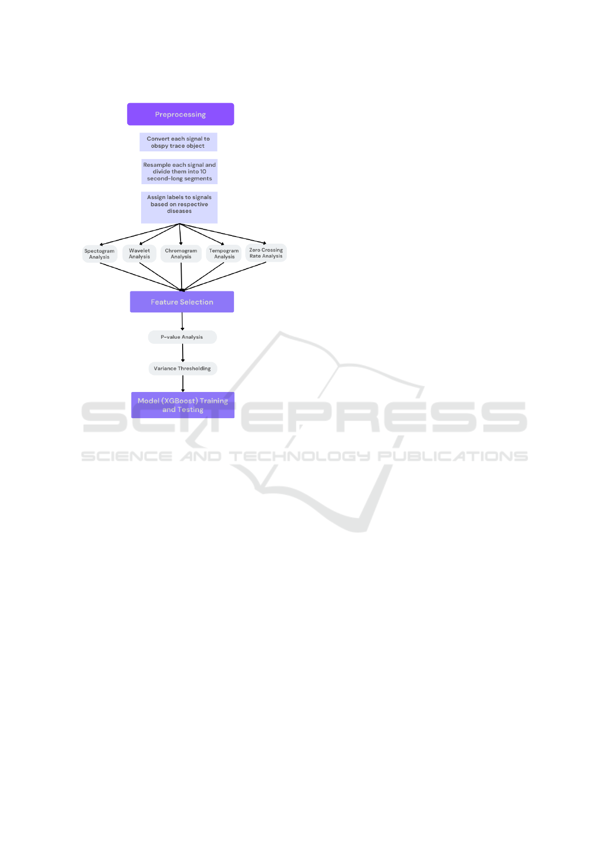
Figure 2: Block diagram for the proposed framework. First,

detrending, tapering, resampling and segmentation were ap-

plied on the signals. Spectrogram, wavelet, chromagram,

tempogram and zero crossing rate features were then ex-

tracted from each segment. Following p-value and vari-

ance thresholding, a multi-label/multi-output classiﬁcation

model was trained and tested using the remaining features.

2.2 Pre-processing of the SCG Signals

As the seismological data and vibrations on the chest

wall have a similar mechanism, SCG signals show

close resemblance to the seismograph signal. Hence,

biomedical signal processing knowledge was com-

bined with the tools available for seismograph anal-

ysis. To that end, the use of ObsPy toolbox, which

allows manipulation and processing of seismograph

signals (Beyreuther et al., 2010), was leveraged. In-

deed, using ObsPy let the SCG signal characteristics

(such as sampling rate, number of points and dura-

tions) be more easily accessible. More importantly,

employment of manual and heuristic pre-processing

and feature extraction methods could be avoided.

Previous studies have shown that SCG analysis

highly beneﬁts from the features extracted from all

three axes (dorso-ventral, lateral and head-to-foot);

hence, in this study, all three axes were included in

the analysis (Semiz et al., 2020). While transform-

ing these signals into traces, each signal was ﬁrst de-

trended linearly to remove unwanted baseline oscilla-

tions. Detrended waveforms were then tapered with

“Hann” window having a decimal percentage of 0.05

to prepare them for frequency analysis. In the dataset,

some signals had a sampling rate of 512 Hz while the

sampling rate for others were 256 Hz. As a solution,

all sampling rates were set to 256 Hz using Obspy’s

resampling method. As the ﬁnal step, each signal was

divided into 10-second long segments to increase the

number of instances. This resulted in a total of 2393

segments (instances).

2.3 Feature Extraction

Following aforementioned pre-processing steps, fea-

ture extraction was performed on the SCG signals. To

that aim, spectrogram, wavelet, chromagram and tem-

pogram features were extracted from each 10-second-

long X, Y, Z segment. Additionally, zero crossing rate

analysis was leveraged as zero crossings were found

correlated with the spectral centroid and dominant

frequencies (Koutroumbas and Theodoridis, 2008).

2.3.1 Spectrogram Analysis

A spectrogram is a two-dimensional function of fre-

quency and time that depicts how a non-stationary

signal’s frequency content changes over time (Mc-

Clellan et al., 2003). Hence, spectrogram analysis

can provide useful information regarding the time-

dependent variances observed in the spectrum.

In this work, spectrogram analysis was employed

using ObsPy’s spectrogram function, with a slight

modiﬁcation in the output. The original function was

outputting the spectrogram images, i.e., the combi-

nation of coefﬁcients, frequency values and time in-

stances. However, for this study, only the spectro-

gram coefﬁcients were required to be used as features.

That is why, time average of the coefﬁcients for each

frequency band was calculated and stored as a vector.

This was repeated for each of the 10-second-long seg-

ment, i. In the end, a matrix S

= (S

x,i

, S

y,i

, S

z,i

) was

generated, which includes time-averaged spectrogram

coefﬁcients for each of the lateral, head-to-foot and

dorso-ventral axes of segment i.

2.3.2 Wavelet Analysis

Physiological signals show time-varying statistics due

to their dynamic nature. As wavelet transform al-

lows for the analysis of non-stationary signals (e.g.

biomedical signals) at multiple scales, it was also

found to be an effective approach for this study. In

BIOSIGNALS 2023 - 16th International Conference on Bio-inspired Systems and Signal Processing

214

wavelet analysis, the signal is decomposed into a col-

lection of basis functions using a ﬁnite-length func-

tion called mother wavelet. Indeed, there are many

different mother wavelets available depending on the

application. The width and central frequency of the

mother wavelet can be adjusted by moving it through

the signal-of-interest. These shifted and scaled ver-

sions of the mother wavelet are also known as daugh-

ter wavelets (Polikar, 1996).

In this work, 1D multilevel discrete wavelet trans-

formation with a level-6 sym5 wavelet was employed.

Having 6 levels ensured that the signal was decom-

posed up until the respiration band (Pandia et al.,

2012). On the other hand, sym5 was chosen as it

shows morphological similarities with the SCG sig-

nals and has been one of the most popular mother

wavelets used in biomedical signal analysis (Jahromi

et al., 2017).

The output was including the approximation co-

efﬁcients (a

) and 6-levels of detail coefﬁcients (d

, d

and d

). Considering that the sam-

pling rate was set to 256 Hz, the maximum frequency

available in the signals was 128 Hz. Thus, the fre-

quency ranges of the detail coefﬁcients were 64-128

Hz, 32-64 Hz, 16-32 Hz, 8-16 Hz, 4-8 Hz, and 2-4

Hz, which correspond to d

, d

and d

co-

efﬁcients, respectively (Fig. 3). On the other hand,

was representing the 0-2 Hz frequency band. The

detail and approximation coefﬁcients were extracted

for all three axes and concatenated together. In the

end, a matrix W

= (W

x,i

, W

y,i

, W

z,i

), was generated,

which includes concatenated approximation and de-

tail coefﬁcients for each of the lateral, head-to-foot

and dorso-ventral axes of segment i.

2.3.3 Chromagram Analysis

In recent years, there have been great advancements in

audio analysis thanks to the semantic analysis (Shah

et al., 2019). Chroma features have found to be pow-

erful representations of any audio as they can be used

to generate audio ﬁngerprints. Chroma features mea-

sure the dominance of the characteristics of a certain

pitch (C, C#, D, D#, E, F, F#, G, G#, A, A# or B)

in signal-of-interest. To compute chroma features,

instantaneous frequency estimates from the spectro-

gram were taken to obtain high-resolution chroma

proﬁles (Giannakopoulos and Pikrakis, 2014).

Recently, it has been shown that biomedical sig-

nal processing can highly beneﬁt from audio anal-

ysis methods, more speciﬁcally from chroma fea-

tures (Hersek et al., 2017). Similarly, in this work,

chroma features corresponding to aforementioned 12

pitch values were extracted from each signal segment.

After extracting pitch values, their time-average was

Figure 3: 6-Level wavelet decomposition. 6-Levels of detail

coefﬁcients: d

, d

and d

. 6

Level approxima-

tion coefﬁcient: a

computed to have one single value for each pitch.

These steps were repeated for all three axes. In the

end, a matrix C

= (C

x,i

, C

y,i

, C

z,i

), was generated

which includes time-averaged pitch values for each

of the lateral, head-to-foot and dorso-ventral axes of

segment i.

2.3.4 Tempogram Analysis

As mentioned in Section 2.3.3, it has been shown

that biomedical signal processing can highly beneﬁt

from audio analysis methods (Hersek et al., 2017).

That is why in addition to chromagram features, tem-

pogram analysis was also leveraged in the analysis.

Tempo and beat, which are components of rhythm,

can be used to distinguish audio from each other.

Unlike beat, tempo can vary locally within an au-

dio. Hence using tempogram, information regarding

tempo at each time instance can be obtained.

From each signal segment, tempogram features

were computed using a hop length and sampling rate

of 256 Hz each. Tempogram coefﬁcients were then

averaged within each window. These steps were again

repeated for all three axes. In the end, a matrix T

x,i

, T

y,i

, T

z,i

), was generated which includes aver-

aged tempogram values for each of the lateral, head-

to-foot and dorso-ventral axes of segment i.

2.3.5 Zero-Crossing Rate Analysis

Zero crossing rate (ZCR) represents the rate of sign-

changes of the signal-of-interest (Giannakopoulos

and Pikrakis, 2014). It is generally used to evaluate

the signal’s noise level, i.e., ZCR values tend to in-

crease as noise levels increases. On the other hand,

ZCR was found to be correlated with the spectral

centroid and dominant frequencies (Koutroumbas and

Theodoridis, 2008). Hence, ZCR value for each seg-

ment was included as a feature in the analysis. For

the 10-second-long segments, ZCR was calculated for

each of the X, Y, Z axes. In the end, a matrix Z

= (z

x,i

y,i

, z

z,i

) was generated where each row refers to one

10-second-long segment, i, and (z

x,i

, z

y,i

, z

z,i

) repre-

Spectral Analysis of Cardiogenic Vibrations to Distinguish Between Valvular Heart Diseases

215

sent the ZCR values of X, Y, Z axes for segment i.

2.3.6 Data Frame Generation

After the aforementioned features were extracted

from each segment, one single data frame was formed

for ease of feature selection and model training. First,

the VHD labels were organized to make the data ready

for multi-label classiﬁcation. To that aim, correspond-

ing VHD label vectors in the form [AR, AS, MR,

MS] were generated and assigned to each 10-second

long segment. The presence of each VHD was la-

beled with 1 and non-presence was indicated with 0.

For example, let us assume that the subject had AR

and MR, however did not have AS or MS. Then the

corresponding label vector was formed as [1,0,1,0].

Similarly if a subject had MS, bu no other VHDs, the

vector was formed as [0,0,0,1]. These label vectors

were generated for each of the 10-second-long seg-

ments, eventually leading to a matrix L, where each

row represents the label vector for one segment.

Following label generation, previously generated

feature matrices and the label matrix were concate-

nated altogether to have one single frame where each

row corresponds to one 10-second long segment. In

the end, the dataframe had the following structure:

, W

, C

, T

, Z

, L

], where S

, W

, C

, T

, Z

, are the

spectrogram, wavelet, chromagram, tempogram and

zero crossing rate features, respectively; and L

is the

corresponding VHD vector for segment i.

2.4 Feature Selection

Following feature extraction, the data frame was in-

cluding 7497 features in total. However this would

cause curse of dimensionality, i.e., the vector space

would be sparser due to an increase in dimension-

ality (Chen, 2009). This would potentially hurt the

training/learning phase and lead to overﬁtting; hence,

multi-step feature selection was employed. First,

Mann-Whitney U test with an alpha level of 0.05 was

applied to the generated dataframe. In other words,

any feature having a p-value smaller than 0.05 was

accepted statistically signiﬁcant. After removing the

features having p > 0.05, variance thresholding was

employed with a threshold of 0.0001. Both methods

are detailed in the following subsections.

2.4.1 p-value Analysis

For p-value-based feature selection, Mann-Whitney

U test with an alpha value of 0.05 was implemented.

Mann-Whitney U test falls under non-parametric hy-

pothesis tests, i.e., it does not make any assumption

regarding the distribution of the data unlike paramet-

ric tests, which assume normal distribution in the

data. Hence, Mann-Whitney U test was determined

as the feature selection method (Sedgwick, 2015).

While performing the test, instead of comparing

the feature variances of the diseases altogether, fea-

tures corresponding to different diseases were com-

pared pair-wise. For example, the spectrogram coefﬁ-

cients of AR were compared with the spectrogram co-

efﬁcients of AS, MR and MS one by one (e.g. ([S

]

vs. [S

]), ([S

] vs. [S

]), ([S

] vs. [S

]),

etc.). This comparison was repeated for all combina-

tions. During each comparison, any feature column

with p value > 0.05 was eliminated and the remain-

ing columns were used in the analysis. As a result,

total number of columns decreased from 7497 to 763.

2.4.2 Variance Thresholding

Following p-value analysis, variance thresholding

was applied on the remaining 763 columns to elim-

inate the redundant features further. Variance thresh-

olding is one of the ﬁlter-based methods and aims to

drop the features having variance values below a pre-

determined threshold (Bommert et al., 2020). Fea-

tures with lower variance indeed carry less informa-

tion, since their variance is proportional to the level

of predictive power they have. Accordingly, the vari-

ance of each feature was calculated and a threshold of

0.0001 was applied. As a result, the total number of

features was decreased from 763 to 308.

2.5 Model Training and Validation

2.5.1 Classiﬁcation Framework and

Performance Metrics

To establish a multi-label/multi-output classiﬁcation

framework, label vectors were generated as previ-

ously explained in Section 2.3.6. The framework was

built using One vs. Rest approach. As the classiﬁ-

cation model, Extreme Gradient Boosting Trees (XG-

Boost) was leveraged. XGBoost falls under ensemble

methods, i.e., instead of a single estimator, multiple

estimators are simultaneously used to predict a vari-

able. During training, multiple decision trees are iter-

atively trained, so that residual errors from the previ-

ous iteration can be predicted and improved over time

(Dietterich et al., 2002).

In this work, 80% of the data was used for training

process and 20% was used for testing. During train-

ing, the objective function was determined to be bi-

nary:logistic, whereas other parameters were kept in

their default values. The performance of the model

was assessed using accuracy, precision, recall, and

BIOSIGNALS 2023 - 16th International Conference on Bio-inspired Systems and Signal Processing

216

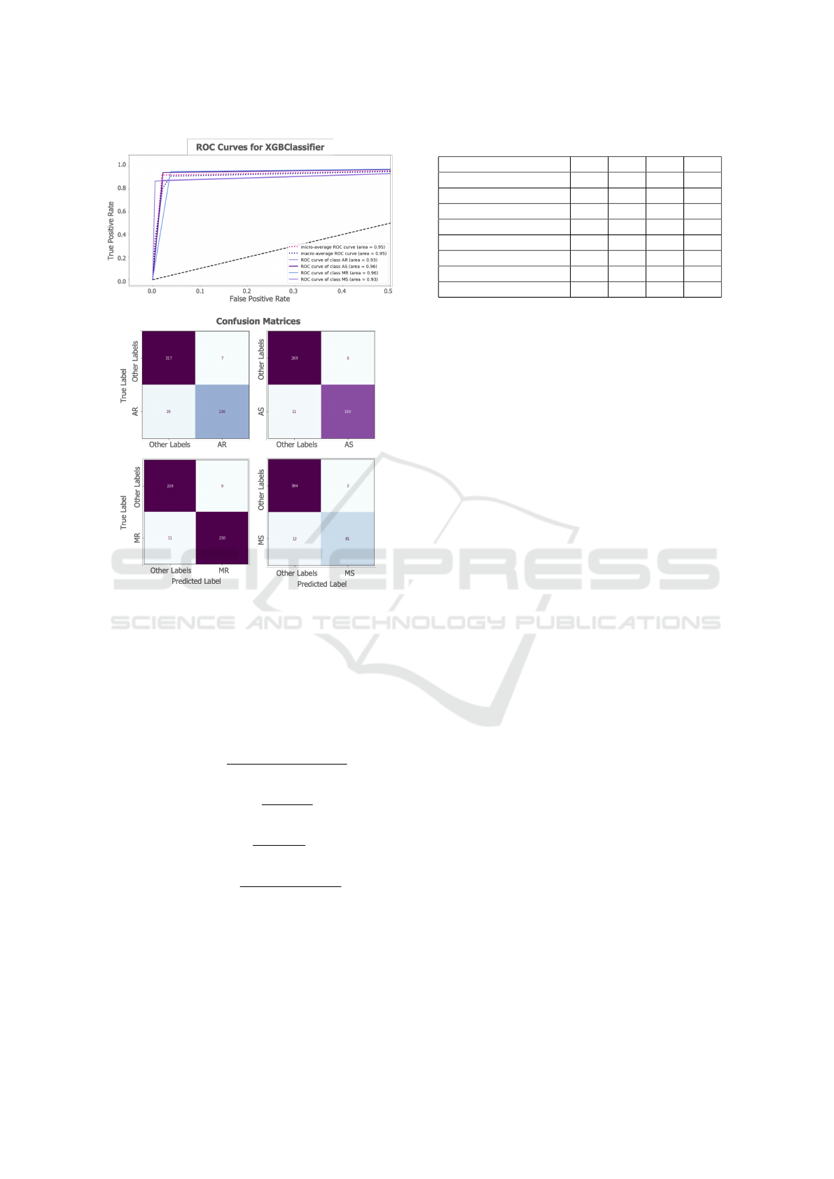
Figure 4: ROC curves and confusion matrices.

f1-score metrics for each of the AR, AS, MR, and

MS classes. The corresponding equations were listed

in Equations 1, 2, 3, 4, respectively (TP: true pos-

itives, FP: false positives, TN: true negatives and

FN: false negatives). In addition, the areas under the

receiver operating characteristics curve (ROC AUC)

were computed for each disease.

Accuracy =

T P + T N

T P + T N + FP + FN

(1)

Precision =

T P

T P + FP

(2)

Recall =

T P

T P + FN

(3)

score = 2 ∗

precision ∗ recall

precision + recall

(4)

2.5.2 Axis Interpretation

As an additional analysis, the X, Y and Z axes fea-

tures were investigated individually to assess the con-

tribution of each axis. To that aim, similar feature

extraction, feature selection and model training steps

Table 2: Classiﬁcation Results.

AR AS MR MS

Accuracy 0.95 0.96 0.96 0.97

Precision (macro) 0.95 0.97 0.96 0.97

Precision (weighted) 0.95 0.96 0.96 0.97

Recall (macro) 0.93 0.96 0.96 0.93

Recall (weighted) 0.95 0.96 0.96 0.97

f1-score (macro) 0.94 0.96 0.96 0.95

f1-score (weighted) 0.95 0.96 0.96 0.97

ROC AUC 0.93 0.96 0.96 0.93

were leveraged, i.e., (i) The spectrogram, wavelet,

tempogram, chromagram and zero crossing rate fea-

tures were ﬁrst assessed using p-value analysis and

variance thresholding. (ii) A multi-label/multi-output

model was then trained and tested using the remain-

ing features. These steps were employed on each of

the X, Y and Z axes. The performance of the models

were again assessed using accuracy, precision, recall,

f1-score and ROC AUC metrics.

3 RESULTS AND DISCUSSION

3.1 Feature Selection

In the ﬁrst part of the analysis, the combination of the

features extracted from all three SCG axes was used.

First, the number of features was decreased from 7497

to 308 using a cascaded feature selection pipeline in-

cluding p-value analysis and variance thresholding.

One important observation was that out of the wavelet

features, only the approximation coefﬁcients, which

correspond to the 0 - 2 Hz, could reject the null hy-

pothesis and be included in the ﬁnal feature set. This

band primarily represents the respiration information

as the frequencies below 1 Hz are associated with the

chest movements originating from exhalation and in-

halation phases (Pandia et al., 2012). In the literature,

it has been shown that respiration has an indisputable

effect on cardiac murmurs as the change in murmur

intensity during breathing can provide valuable infor-

mation regarding the origin and pathological signif-

icance of the murmur (Levin et al., 1962). Hence,

these ﬁndings were indeed consistent with the under-

lying physiological processes. Another important ob-

servation was that all zero-crossing-rate features from

all three axes could reject the null hypothesis, thus

it can be deduced that different VHDs induce differ-

ent amounts of sign change on the SCG signals. This

difference can be attributed to either the differences

in induced noise or effects on spectral components as

previously discussed (Giannakopoulos and Pikrakis,

2014; Koutroumbas and Theodoridis, 2008).

Spectral Analysis of Cardiogenic Vibrations to Distinguish Between Valvular Heart Diseases

217

Table 3: Performance Metrics for X, Y, Z axes individually.

X (lateral) Y (head-to-foot) Z (dorso-ventral)

AR AS MR MS AR AS MR MS AR AS MR MS

Accuracy 0.92 0.91 0.90 0.93 0.91 0.90 0.90 0.93 0.92 0.93 0.92 0.95

Precision (macro) 0.92 0.91 0.90 0.91 0.92 0.90 0.90 0.90 0.93 0.93 0.92 0.95

Precision (weighted) 0.92 0.91 0.90 0.93 0.91 0.90 0.90 0.92 0.92 0.93 0.92 0.95

Recall (macro) 0.89 0.90 0.90 0.86 0.87 0.90 0.90 0.86 0.90 0.92 0.92 0.88

Recall (weighted) 0.92 0.91 0.90 0.93 0.91 0.90 0.90 0.93 0.92 0.93 0.92 0.95

f1-score (macro) 0.91 0.90 0.90 0.89 0.89 0.90 0.90 0.88 0.91 0.93 0.92 0.91

f1-score (weighted) 0.92 0.91 0.90 0.93 0.90 0.90 0.90 0.93 0.92 0.93 0.92 0.95

ROC AUC 0.89 0.90 0.90 0.86 0.87 0.90 0.90 0.86 0.89 0.92 0.92 0.88

3.2 Classiﬁcation Results

Following feature elimination, an XGBoost-based

multi-label/multi-class classiﬁcation framework

leveraging One vs. Rest strategy was built. To assess

the model performance, accuracy, precision, recall,

f1-score and ROC AUC metrics were calculated.

The multi-label/multi-class classiﬁcation results,

corresponding ROC curves and confusion matrices

for each VHD are presented in Table 2 and Fig. 4.

As seen, for all four VHDs, the accuracy, weighted

precision, weighted recall and weighted f1-score

values were above 95%. Additionally, the average

ROC AUC value for all four VHDs was calculated

as 0.95 (Fig. 4). Obtaining superior performance

values shows that the spectral features and the

XGBoost-based multi-label/multi-class classiﬁcation

framework work at sufﬁciently high performance.

3.3 Axis Interpretation

As the last analysis, the aforementioned analysis

pipeline was repeated on the X, Y and Z axes indi-

vidually. Initially, there were 2499 features extracted

from each of the lateral (X), head-to-foot (Y), and

dorso-ventral (Z) axes. For the X axis, this num-

ber decreased to 252 following p-value analysis and

to 143 after variance thresholding. Similarly for Y

and Z axes, these values were 256 to 131 and 253 to

159, respectively. For each axis, a separate model was

trained and tested. The multi-label/multi-class classi-

ﬁcation results are presented in Table 3. As expected,

the classiﬁer performances were lower compared to

the case where features from all three axes were used,

however still most of the performance values were

above 90%. The best performing axis was found to

be the dorso-ventral direction (Z), which has indeed

been the most commonly used axis in cardiovascular

health assessment (Taebi et al., 2019).

4 CONCLUSIONS

In this paper, an XGBoost-based multi-label/multi-

class classiﬁcation framework was proposed to dis-

tinguish between aortic stenosis (AS), aortic valve

regurgitation (AR), mitral valve stenosis (MS), and

mitral valve regurgitation (MR) using the tri-axial

SCG signals collected from the mid-sternum. First,

seismology domain knowledge was leveraged and

applied to SCG signals through ObsPy toolbox for

pre-processing. From pre-processed signal segments,

spectrogram, wavelet, chromagram, tempogram and

zero-crossing-rate features were extracted. Following

p-value analysis and variance thresholding, a multi-

label/multi-class classiﬁcation framework based on

gradient boosting trees was developed to distinguish

between AS, AR, MS and MR cases.

For all four VHDs, the accuracy, weighted pre-

cision, weighted recall and weighted f1-score values

were above 95%. In addition, when the SCG axes

were investigated individually, it was found that the

features extracted from the dorso-ventral direction (Z

axis) shows superior performance compared to other

two axes. Overall, the results showed that spectral

analysis of SCG signals can provide valuable infor-

mation regarding VHDs and potentially be used in

the design of continuous monitoring systems. Future

work will focus on validating these ﬁndings in larger

datasets and improving the current pipelines further

to achieve real-time VHD detection and assessment.

REFERENCES

Beyreuther, M., Barsch, R., Krischer, L., Megies, T., Behr,

Y., and Wassermann, J. (2010). Obspy: A python tool-

box for seismology. Seismological Research Letters,

81(3):530–533.

Bommert, A., Sun, X., Bischl, B., Rahnenf

uhrer, J., and

Lang, M. (2020). Benchmark for ﬁlter methods

for feature selection in high-dimensional classiﬁca-

BIOSIGNALS 2023 - 16th International Conference on Bio-inspired Systems and Signal Processing

218

tion data. Computational Statistics & Data Analysis,

143:106839.

Chen, L. (2009). Curse of dimensionality. encyclopedia of

database systems.

Dietterich, T. G. et al. (2002). Ensemble learning.

The handbook of brain theory and neural networks,

2(1):110–125.

Giannakopoulos, T. and Pikrakis, A. (2014). Introduction

to audio analysis: a MATLAB® approach. Academic

Press.

Go, A. S., Mozaffarian, D., Roger, V. L., Benjamin, E. J.,

Berry, J. D., Borden, W. B., Bravata, D. M., Dai, S.,

Ford, E. S., Fox, C. S., et al. (2013). Heart disease

and stroke statistics—2013 update: a report from the

american heart association. Circulation, 127(1):e6–

e245.

Golubnitschaja, O., Kinkorova, J., and Costigliola, V.

(2014). Predictive, preventive and personalised

medicine as the hardcore of ‘horizon 2020’: Epma po-

sition paper. EPMA Journal, 5(1):1–29.

Hersek, S., Pouyan, M. B., Teague, C. N., Sawka, M. N.,

Millard-Stafford, M. L., Kogler, G. F., Wolkoff, P.,

and Inan, O. T. (2017). Acoustical emission analysis

by unsupervised graph mining: A novel biomarker of

knee health status. IEEE Transactions on Biomedical

Engineering, 65(6):1291–1300.

Hurnanen, T., Lehtonen, E., Tadi, M. J., Kuusela, T.,

Kiviniemi, T., Saraste, A., Vasankari, T., Airaksinen,

J., Koivisto, T., and P

ank

a, M. (2016). Auto-

mated detection of atrial ﬁbrillation based on time–

frequency analysis of seismocardiograms. IEEE jour-

nal of biomedical and health informatics, 21(5):1233–

1241.

Imirzalioglu, M. and Semiz, B. (2022). Quantifying respira-

tion effects on cardiac vibrations using teager energy

operator and gradient boosted trees. In 2022 44th An-

nual International Conference of the IEEE Engineer-

ing in Medicine & Biology Society (EMBC), pages

1935–1938. IEEE.

Inan, O. T., Baran Pouyan, M., Javaid, A. Q., Dowling, S.,

Etemadi, M., Dorier, A., Heller, J. A., Bicen, A. O.,

Roy, S., De Marco, T., et al. (2018). Novel wearable

seismocardiography and machine learning algorithms

can assess clinical status of heart failure patients. Cir-

culation: Heart Failure, 11(1):e004313.

Inan, O. T., Migeotte, P.-F., Park, K.-S., Etemadi, M.,

Tavakolian, K., Casanella, R., Zanetti, J., Tank, J.,

Funtova, I., Prisk, G. K., et al. (2014). Ballistocardio-

graphy and seismocardiography: A review of recent

advances. IEEE journal of biomedical and health in-

formatics, 19(4):1414–1427.

Jahromi, M. G., Parsaei, H., Zamani, A., and Dehbozorgi,

M. (2017). Comparative analysis of wavelet-based

feature extraction for intramuscular emg signal de-

composition. Journal of biomedical physics & engi-

neering, 7(4):365.

Klabunde, R. (2011). Cardiovascular physiology concepts.

Lippincott Williams & Wilkins.

Koutroumbas, K. and Theodoridis, S. (2008). Pattern

recognition. Academic Press.

Lay, T. and Wallace, T. C. (1995). Modern global seismol-

ogy. Elsevier.

Levin, H. S., Runco, V., Goodwin, R. S., Ryan, J. M., et al.

(1962). The effect of respiration on cardiac murmurs:

An auscultatory illusion. The American Journal of

Medicine, 33(2):236–242.

McClellan, J. H., Schafer, R. W., and Yoder, M. A. (2003).

Signal processing ﬁrst. Pearson education Upper Sad-

dle River, NJ.

Meister, S., Deiters, W., and Becker, S. (2016). Digital

health and digital biomarkers–enabling value chains

on health data. Current Directions in Biomedical En-

gineering, 2(1):577–581.

Pandia, K., Inan, O. T., Kovacs, G. T., and Giovangrandi, L.

(2012). Extracting respiratory information from seis-

mocardiogram signals acquired on the chest using a

miniature accelerometer. Physiological measurement,

33(10):1643.

Polikar, R. (1996). The wavelet tutorial second edition

part i. Fundamental Concepts & An Overview of The

Wavelet Theory.

Sedgwick, P. (2015). A comparison of parametric and non-

parametric statistical tests. BMJ, 350.

Semiz, B., Carek, A. M., Johnson, J. C., Ahmad, S.,

Heller, J. A., Vicente, F. G., Caron, S., Hogue, C. W.,

Etemadi, M., and Inan, O. T. (2020). Non-invasive

wearable patch utilizing seismocardiography for peri-

operative use in surgical patients. IEEE Journal

of Biomedical and Health Informatics, 25(5):1572–

1582.

Shah, A., Kattel, M., Nepal, A., and Shrestha, D. (2019).

Chroma feature extraction. Chroma Feature Extrac-

tion using Fourier Transform.

Shandhi, M. M. H., Semiz, B., Hersek, S., Goller, N.,

Ayazi, F., and Inan, O. T. (2019). Performance

analysis of gyroscope and accelerometer sensors for

seismocardiography-based wearable pre-ejection pe-

riod estimation. IEEE journal of biomedical and

health informatics, 23(6):2365–2374.

Svensson, L. (2008). Aortic valve stenosis and regurgita-

tion: an overview of management. Journal of Cardio-

vascular Surgery, 49(2):297.

Taebi, A., Solar, B. E., Bomar, A. J., Sandler, R. H., and

Mansy, H. A. (2019). Recent advances in seismocar-

diography. Vibration, 2(1):64–86.

WHO (2020). The top 10 causes of death. Geneva: World

Health Organization. https://www.who.int/news-

room/fact-sheets/detail/the-top-10-causes-of-death

(visited: 2022-09).

Yang, C., Aranoff, N. D., Green, P., and Tavassolian, N.

(2019). Classiﬁcation of aortic stenosis using time–

frequency features from chest cardio-mechanical sig-

nals. IEEE Transactions on Biomedical Engineering,

67(6):1672–1683.

Yang, C., Fan, F., Aranoff, N., Green, P., Li, Y., Liu, C., and

Tavassolian, N. (2021). An open-access database for

the evaluation of cardio-mechanical signals from pa-

tients with valvular heart diseases. Frontiers in Phys-

iology, 12.

Spectral Analysis of Cardiogenic Vibrations to Distinguish Between Valvular Heart Diseases

219