Flow-Based Visual-Inertial Odometry for Neuromorphic Vision Sensors

Using non-Linear Optimization with Online Calibration

Mahmoud Z. Khairallah

∗ a

, Abanob Soliman

∗ b

, Fabien Bonardi

† c

, David Roussel

† d

and Samia Bouchafa

† e

Universit

e Paris-Saclay, Univ. Evry, IBISC Laboratory, 34 Rue du Pelvoux, Evry, 91020, Essonne, France

∗

ﬁ ﬁ

Keywords:

Neuromorphic Vision Sensors, Optical Flow Estimation, Visual-Inertial Odometry.

Abstract:

Neuromorphic vision sensors (also known as event-based cameras) operate according to detected variations in

the scene brightness intensity. Unlike conventional CCD/CMOS cameras, they provide information about the

scene with a very high temporal resolution (in the order of microsecond) and high dynamic range (exceeding

120 dB). These mentioned capabilities of neuromorphic vision sensors induced their integration in various

robotics applications such as visual odometry and SLAM. The way neuromorphic vision sensors trigger events

is strongly coherent with the brightness constancy condition that describes optical ﬂow. In this paper, we

exploit optical ﬂow information with the IMU readings to estimate a 6-DoF pose. Based on the proposed

optical ﬂow tracking method, we introduce an optimization scheme set up with a twist graph instead of a

pose graph. Upon validation on high-quality simulated and real-world sequences, we show that our algorithm

does not require any triangulation or key-frame selection and can be ﬁne-tuned to meet real-time requirements

according to the events’ frequency.

1 INTRODUCTION

By providing frame-free asynchronous data, event-

based cameras are designed to trigger events and re-

act to changes in brightness in the scene whenever de-

tected. These sensors are designed to mimic the activ-

ities of the biological retina and do not depend on any

artiﬁcial clock signals. The asynchronous nature of

event-based cameras enables them to suppress redun-

dant data (compared to frame-based cameras), pro-

vide high temporal resolution and high dynamic range

with low power consumption. These sensors provide

a convenient replacement for frame-based vision sen-

sors in scenarios presenting high dynamics such as

drone motion.

For the past decade, many solutions have been in-

troduced to integrate event-based cameras in robotic

applications: for instance, (Kim et al., 2008), (Mueg-

gler et al., 2014), (Rebecq et al., 2017a) and (Mueg-

gler et al., 2018) provide accurate motion estimation.

Amongst the adopted approaches to solve this prob-

lem, different probabilistic ﬁltering methods have

https://orcid.org/0000-0002-0724-8450

https://orcid.org/0000-0003-4956-8580

https://orcid.org/0000-0002-3555-7306

https://orcid.org/0000-0002-1839-0831

https://orcid.org/0000-0002-2860-8128

been introduced in (Kim et al., 2008), (Kim et al.,

2016), (Weikersdorfer and Conradt, 2012) and (Weik-

ersdorfer et al., 2013). Other methods like (Mueggler

et al., 2014), (Kueng et al., 2016) and (Weikersdorfer

et al., 2014) used different optimization schemes to

beneﬁt from their higher accuracy to estimate motion.

Event-based cameras’ ability to provide asyn-

chronous data with signiﬁcantly high temporal reso-

lution leads to better continuous representation com-

pared to frame-based cameras, as well as eliminating

other problems such as motion blur and low dynamic

range. Furthermore, this ability provides a more sta-

ble mathematical modeling of the brightness con-

stancy condition, which describes the apparent pixels

motion known as the optical ﬂow. In this paper, we

introduce, to the extent of our knowledge, the ﬁrst

visual-inertial odometry algorithm that jointly opti-

mizes the events’ optical ﬂow with the inertial mea-

surements for neuromorphic vision sensors.

2 RELATED WORK

The change in vision sensors nature proposed by

event-based cameras required a paradigm shift on

how the visual odometry problem is modeled and how

it can be solved. During the past decade, many at-

Khairallah, M., Soliman, A., Bonardi, F., Roussel, D. and Bouchafa, S.

Flow-Based Visual-Inertial Odometry for Neuromorphic Vision Sensors Using non-Linear Optimization with Online Calibration.

DOI: 10.5220/0011660400003417

In Proceedings of the 18th International Joint Conference on Computer Vision, Imaging and Computer Graphics Theory and Applications (VISIGRAPP 2023) - Volume 5: VISAPP, pages

963-973

ISBN: 978-989-758-634-7; ISSN: 2184-4321

 2023 by SCITEPRESS – Science and Technology Publications, Lda. Under CC license (CC BY-NC-ND 4.0)

963

tempts were introduced where some adapted the ac-

quired data from event-based cameras to suit frame-

based algorithms (Gehrig et al., 2020; Muglikar et al.,

2021) in order to create frames from event-based cam-

eras, while others reformulated the problem to fully

exploit event-based capabilities (Zhou et al., 2021;

Rebecq et al., 2017a; Rebecq et al., 2018). A novel

method was presented in (Weikersdorfer and Conradt,

2012) using a particle ﬁlter for motion tracking to es-

timate the camera’s rotation by creating mosaic im-

ages of the scene, while an extended Kalman ﬁlter is

used to reﬁne the gradient intensity results. In (Weik-

ersdorfer et al., 2013), a particle ﬁlter is used to es-

timate the 2D motion of the used rig based on the

work presented in (Weikersdorfer and Conradt, 2012)

and a 2D map is simultaneously reconstructed. Mueg-

gler et al. (Mueggler et al., 2014) developed a 6-DoF

motion estimation for simple, uncluttered and struc-

tured environments that contain lines where the pose

is estimated by minimizing the reprojection error of

each detected line in the environment. Rebecq et al.

(Rebecq et al., 2017a) proposed an event-based track-

ing and mapping method to estimate the pose based

on image alignment by warping event images using

Lucas-Kanade method (Baker and Matthews, 2004)

and constructed the map thanks to the event-based

space-sweep presented in (Rebecq et al., 2018) to pro-

vide depth and 3D map. Kim et al. (Kim et al., 2016)

pursued their work in (Kim et al., 2008) using an ex-

tended Kalman ﬁlter to estimate pose, gradient inten-

sity and mapping implemented using a GPU.

Enhancing the robustness and accuracy of algo-

rithms using event-based cameras can be done, sim-

ilarly to frame-based cameras, by augmenting the

camera with either a different kind of sensor such

as frame-based RGB-D cameras, or another event-

based camera for stereo-vision. Censi and Scara-

muzza (Censi and Scaramuzza, 2014) provided 6-

DoF visual odometry by fusing the event-based cam-

era with a CMOS camera where only rotation was ac-

curately estimated and translation suffered from a de-

teriorated accuracy. Kueng et al. (Kueng et al., 2016)

tracked the features detected in a CMOS image frame

using the event-based camera and used a Bayesian

depth ﬁlter to estimate the depth of 2D tracked fea-

tures and obtain 3D points. These 3D points are then

used to minimize the reprojection error between 2D

features and 3D points to estimate 6-DoF pose. Weik-

ersdorfer et al. (Weikersdorfer et al., 2014) used an

extrinsically calibrated RGB-D sensor with an event-

based camera to provide an accurate transformation

of each depth value in the events’ frame and applied a

Bayesian particle ﬁlter to estimate 6-DoF pose and a

map.

Using an Inertial Measurement Unit (IMU) helps

to improve estimates provided by a monocular cam-

era to obtain accurate absolute scale. Zihao et al. (Zi-

hao Zhu et al., 2017) track features using optical-ﬂow-

based expectation maximization to warp features and

then use the tracked features with IMU measurements

in a structure-less Kalman ﬁlter scheme for pose esti-

mation. Mueggler et al. (Mueggler et al., 2018) used

splines on a manifold for better representation of IMU

readings and minimized the geometric reprojection

and IMU error for 6-DoF pose estimation. Vidal et

al. (Vidal et al., 2018) proposed a SLAM

system that

combines an event-based camera, CMOS camera and

an IMU to provide an accurate scheme based on pre-

vious work (Rebecq et al., 2017b) which mainly de-

pends on feature tracking and non-linear key-frames

optimization. (Le Gentil et al., 2020) exploited the ge-

ometric structure of the environment and developed a

visual-inertial system that exploits the detected lines

instead of evens in the scene to estimate ego-motion.

State-of-the-art algorithms presented in the liter-

ature of event-based cameras vary in their approach,

estimated states, used sensors and performance. De-

spite the fact that event-based cameras adopt a mode

of operation that differs from frame-based cameras,

the introduced algorithms mainly depend on concepts

embraced for frame-based techniques such as fea-

tures extraction and key-frames optimization and tri-

angulation. Moreover, the event-based change detec-

tion model and the high temporal resolution of event-

based cameras highly improved the quality of optical

ﬂow estimation. Although optical ﬂow incorporates

6-DoF information (Longuet-Higgins and Prazdny,

1980; Zucchelli et al., 2002), we observe that opti-

cal ﬂow is not fully exploited in event-based 6-DoF

estimation except for some image warping tasks (Zi-

hao Zhu et al., 2017).

In this paper, we introduce a visual-inertial odom-

etry optimization scheme that essentially depends on

optical ﬂow information corrected using the IMU

measurements. The following Section presents Neu-

romorphic Vision and how an event is triggered.

Section 4 demonstrates how visual-inertial odometry

works and illustrates our optimization scheme. The

experimental setup required to validate our scheme is

shown in Section 5 and the obtained results in Section

Simultaneous Localization And Mapping

VISAPP 2023 - 18th International Conference on Computer Vision Theory and Applications

964





 



 



 

 









 

 





 



 



 



 



 

 





 



 



 

 

   







 



 



 



 



 

 

 

 







 





 









 





 



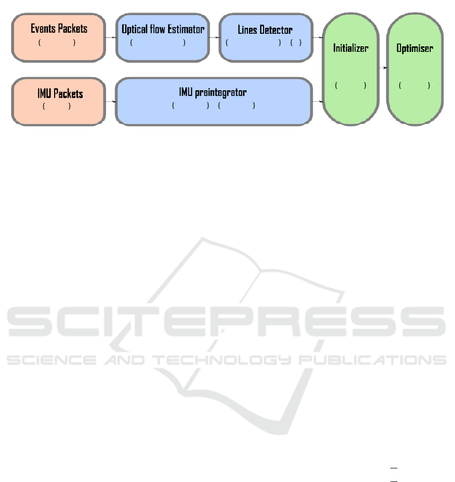
Figure 1: Optical Flow (OF) based visual-inertial odometry scheme where each block shows its expected output. In red: Raw

data, green: processed data required for optimization, blue: The optimization scheme and the initializer outputting 6-DoF

Pose, twist and line depth.

3 NEUROMORPHIC VISION

MODEL

Rather than providing complete frames at regular in-

tervals, each pixel of an event-based camera gener-

ates an asynchronous ﬂow of events. The generated

ﬂow is triggered whenever a change in light inten-

sity is detected. An event e

= {x, y, p,t} is described

by its pixel position (x, y), its polarity p ∈ {−1, 1}

and the timestamp of the event t. Whenever light

intensity variation on a pixel exceeds the threshold

∈ [10%, 15%], an event is triggered according to

the equation:

∆L(x

) = L(x

) − L(x

− ∆t) = p

(1)

where, for each pixel (x

), L(x

) and

L(x

− ∆t) are the light intensity log at time t

and earlier time t

− ∆t. The triggered event e has a

±1 polarity based on the increase or the decrease of

light intensity ±∆L.

4 FLOW-BASED

VISUAL-INERTIAL

ODOMETRY

4.1 Preliminaries

4.1.1 Pose

Vision-based 6-DoF state estimation algorithms in-

crementally estimate a 6-DoF pose T ∈ SE(3) deﬁned

as the rigid body transformation. A rigid body trans-

formation T

i j

expressed as a Lie group L differen-

tiable on manifold with the Lie algebra A as its tan-

gent space at the identity is called a twist ζ

i j

. The

logarithmic map Log : L → A is used to obtain the

twist ζ

i j

of T

i j

at the identity space and its inverse

can be found using the exponential map Exp : A → L

(Chirikjian, 2011).

i j



i j

0 1



, ζ

i j



⌊Ω

i j

⌋

i j

0 1



, (2)

where R

i j

∈ SO(3) is the rotational matrix, t

i j

∈ R

is the translation vector, ⌊Ω

i j

⌋

∈ so(3) is the skew

symmetric matrix of the angular velocity vector and

i j

∈ R

is the linear velocity vector. The vec-

tor space representing the rigid body transformation

(group and algebra) is represented by the vee operator

(.)

∨

: L,A → R

and is reversed by the hat operator

(.)

∧

4.1.2 Pinhole Model

Event-based cameras uses the pinhole model (Cy-

ganek and Siebert, 2011) (or any reprojection model

according to the used lens) to describe the 3D/2D

projection π : R

→ R

of any 3D point X

]

∈ R

in the camera frame to a 2D point

= [x

]

∈ R

on the image plane as:



]







+ c

(3)

where ( f

, f

) are the lens focal length values and

) are the the principal point coordinates in x

and y directions, respectively. The pinhole model is a

planar model which requires each pixel (event in our

case) to be undistorted for accurate 3D/2D projection.

4.1.3 Optical Flow Representation

Optical ﬂow describes the pixels apparent motion

(Longuet-Higgins and Prazdny, 1980) which can

be approximated as the perspective projection of

a 3D point X

moving freely with linear veloc-

ity V

= [v

]

and angular velocity Ω

Flow-Based Visual-Inertial Odometry for Neuromorphic Vision Sensors Using non-Linear Optimization with Online Calibration

965

[ω

,ω

]

so that the point’s 3D velocity is de-

scribed as:

= −(Ω

× X

) =









= −









−Y

− Z

− X

















(4)

2D point velocities (optical ﬂow approximation) cor-

responding to the optical ﬂow can be obtained by the

derivative of Equation (3) incorporating (4):

˙x





−

A(x

+B(x

)Ω

(5)

where the matrices A and B are function of image

plane coordinates:

A =



− f 0 (x

− c

)

0 − f (y

− c

)



B =





−c

)(y

−c

)

−



f +

−c

)



− c

)



f +

−c

)



−

−c

)(y

−c

)

−(x

− c

)





(6)

Hence, estimating the optical ﬂow, if the twist vector

∨

is known, would require also knowledge about the

depth Z

of each point.

4.1.4 IMU Preintegration Measurements

An inertial measurement unit provides proprioceptive

information as the linear acceleration

(t) and angu-

lar velocity

Ω

(t) expressed in the body frame and

inﬂuenced by different noise sources described as:

Ω

(t) = Ω

(t) + b

(t) + η

(t) (7)

(t) = a

(t) + R

g + b

(t) + η

(t) (8)

where η

(t) and η

(t) are the Gaussian white noise of

the IMU random walk characterised as N (0,σ

) and

N (0, σ

), respectively. Ω

(t) and a

(t) are the actual

angular velocity and linear acceleration of the IMU,

is the rotation matrix between the body frame and

the world frame and g is the gravity vector. b

(t) and

(t) are the slowly varying random walk noise of the

sensors with their rates deﬁned by:

(t) = η

(9)

where η

and η

are the Gaussian white noise

of the IMU biases characterised as N (0, σ

) and

N (0, σ

), respectively.

Estimating the states of motion from an instant i to the

instant j is done by integrating the linear acceleration

and angular velocity:

) =R

)Exp



(

Ω(τ) − b

(τ) − η

(τ))dτ



(10)

) =V

) +

(

a(τ) − b

(τ) − η

(τ)) − g)dτ

(11)

) =P

) +V

i j

)∆t

(

a(τ) − b

(τ) − η

(τ)) − g) dτ

(12)

where R

is the rotation matrix, V

is the velocity

vector and P

is the position vector. Instead of using

equations 10, 11 and 12 which would slow down op-

timization and increase estimation errors, we adopt a

preintegration representation of IMU measurements

introduced in (Lupton and Sukkarieh, 2011) and

modiﬁed for representation on manifolds in (Forster

et al., 2016) to avoid recomputation of parameters.

Preintegration provides the increments of the state

} between two time steps i and j ex-

pressed as:

∆R

i j

) = ∆

i j

)Exp(−δφ

i j

), (13)

∆V

i j

) = ∆

i j

) − δV

i j

), (14)

∆P

i j

) = ∆

i j

) − δP

i j

), (15)

where ∆(.) represent the difference of the state be-

tween the two time steps i and j,

(.) means that the

states are estimated directly from measurements with

no noise estimation, δ(.) denotes the preintegration

values of the rotation, velocity and position states in-

corporating the IMU noise propagation and deﬁned in

the method given in (Forster et al., 2016).

4.2 Optimization Scheme

Using the optical ﬂow for accurate motion estima-

tion is a complex problem which requires, in some

cases, decoupling the translational and rotational mo-

tion and a prior knowledge of depth (Zucchelli, 2002;

Liu et al., 2017). In a different approach, we exploit

the geometric characteristics of the environment be-

sides augmenting the optical ﬂow with IMU measure-

ments to obtain accurate ego-motion and depth esti-

mation (see Figure 1). In order to have reliable event-

based optical ﬂow estimation with acceptable com-

putational time, we used a PCA event-based optical

VISAPP 2023 - 18th International Conference on Computer Vision Theory and Applications

966

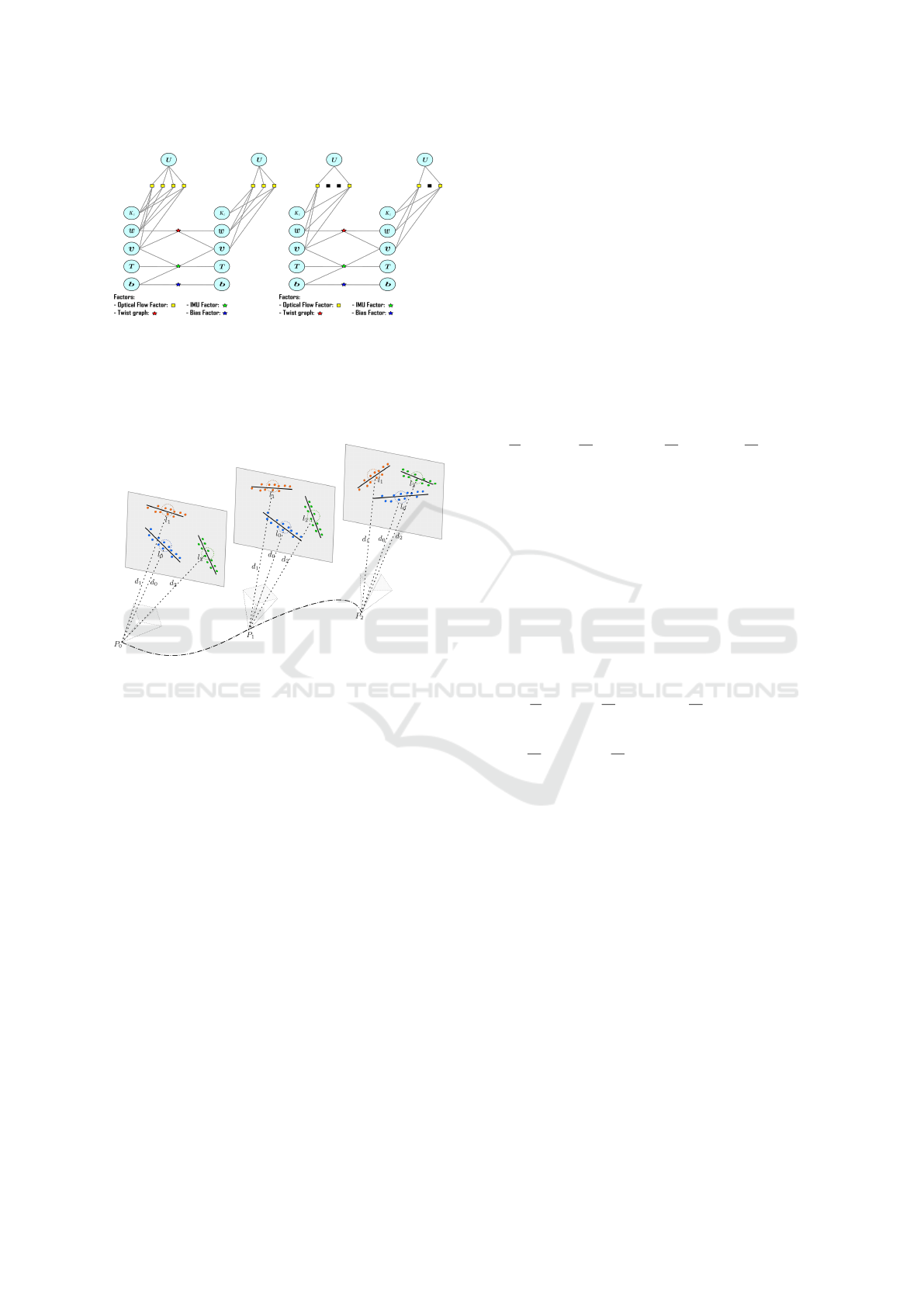
(a) (b)

Figure 2: A) Factor graph with no dropped events between

two optimization time steps, b)Factor graph where some

events are dropped. In case of dropping events, the number

of Optical Flow edges decrease, and accordingly the total

optimization time is reduced signiﬁcantly.

Figure 3: A conceptional drawing of different detected lines

at different time steps with their assigned events with a

small radius around the center point. We choose only events

around the center with their optical ﬂow to participate in the

initial depth estimation assuming small depth variation.

ﬂow approach (Khairallah et al., 2022b) where each

event’s information becomes {x,y, p,t,u, v} with the

optical ﬂow u and v in x and y directions.

Event-Based cameras provide signals due to

changes in the environment which would occur on

contours of objects. This makes Event-Based sensors

suitable for semi-dense SLAM and visual odometry

algorithms. We beneﬁt from the richness of events

creating contours in structured environments to de-

tect and track lines using a ﬂow-based line detector

(Khairallah et al., 2022a).

In our scheme, we follow a probabilistic approach

exploiting optical ﬂow and detected lines (Furgale

et al., 2012). We obtain optimal state estimates X (t)

within a time interval of [t

] using a set of measure-

ments Z(t) where the environment has the structure

S in a joint posterior estimate p(X (t)|Z(t)) with no

map or prior belief. The set of measurements consist

of measured optical ﬂow given the position of each

event U

(t), the accelerometer measurements A(t)

and gyroscope measurements W (t). With no prior

belief, we try to ﬁnd a maximum likelihood of mea-

surements using the estimated states as:

p(X (t)|U

(t),A(t), W (t))

= p(X (t)|U

(t))p(X (t)|A(t))p(X (t)|W (t))

(16)

where the conditional probability of Equation (16)

consists of the multiplication of conditional probabil-

ities of measurements given that each set of measure-

ments is independent of the others. We assume that

each conditional probability is described as a Gaus-

sian probability distribution with zero mean and a

variance σ. Obtaining the maximum likelihood is

equivalent to estimating the minimum of the log func-

tion which is expressed as the following cost function:

F =

∑

i=1

∆

∑

i=1

∆

jimu

∑

i=1

∆

jba

∑

i=1

∆

jbw

(17)

Where N is the number of events providing optical

ﬂow during optimization span and M is the number

of IMU measurements used. ∆

, ∆

jimu

are the error

terms corresponding to optical ﬂow estimation, IMU

measurements, respectively. ∆

jba

and ∆

jbw

are the er-

ror terms corresponding to the accelerometer and gy-

roscope bias. In order to enhance the optimization

process we added a twist error term ∆

jζ

responsible

for reﬁning the twist used for optical ﬂow estimation

(see Figure 2). The new enhanced robust objective

function is deﬁned as:

F =

∑

i=1

∆

∑

i=1

∆

jimu

∑

i=1

∆

jba

∑

i=1

∆

jbw

∑

i=1

∆

jζ

(18)

Where ρ denotes the Huber norm (Huber, 1992).

The optical ﬂow error ∆

is deﬁned as:

∆

= (u

(t) − u

(d(t)))

(t)−u

(d(t))) (19)

where Σ

is the covariance matrix associated with

the optical ﬂow. u

(t) is the estimated optical ﬂow,

(d(t)) is the measured optical ﬂow using the IMU

measurements (see Equation (5)) where the depth Z

initial estimate is shown in the initialization step (see

Section 4.3.1). To alleviate the problem of estimating

the depth of each event independently – which would

require heavier computations – and since the provided

events are created due to the motion of contours of

objects, we assumed that the environment contains a

sufﬁcient amount of contour lines that can be used to

estimate the depth.

The IMU measurements error term ∆

imu

is deﬁned

as:

∆

imu

= [∆

Ri j

,∆

vi j

,∆

pi j

]

imu

[∆

Ri j

,∆

vi j

,∆

pi j

] (20)

Flow-Based Visual-Inertial Odometry for Neuromorphic Vision Sensors Using non-Linear Optimization with Online Calibration

967

where Σ

imu

is the IMU covariance matrix. The prein-

tegration error terms are:

∆

Ri j

= Log



∆

i j

Exp



∂

∂b



)

∆

vi j

= R



−V

− g∆t

i j



−



∆

i j

∂

∂b

∂

∂b



∆

pi j

= R



− P

−V

∆t

i j

−

g∆t

i j



−



∆

i j

∂

∂b

∂

∂b



(21)

where the partial derivatives [

∂

∂b

∂

∂b

∂

∂b

∂

∂b

∂

∂b

]

are calculated as explained in the supplementary ma-

terials of (Forster et al., 2016).

The error terms for the biases ∆

and ∆

are deﬁned

as:

∆

= (b

a j

− b

)

a j

− b

), (22)

∆

= (b

w j

− b

)

w j

− b

). (23)

The twist error term as:

∆

ζi j



∆t

−1



⊖ ζ

i j





∆t

−1



⊖ ζ

i j



(24)

Frame-based optimization schemes using features

choose certain key-frames to achieve triangulation

with low uncertainty. Conversely, using optical ﬂow

allows to ignore key-frames and freely choose the

time steps for optimization depending on either the

number of events N or the number of IMU read-

ings M. Moreover, having rich events optical ﬂow

and lines ensure we can drop events whenever events

frequency exceeds a threshold in order to main-

tain real-time processing. The state vector we op-

timize contains position, rotation quaternion, veloc-

ity, IMU biases and the camera intrinsic parameters

{P,Q,V , d, b

}, where Q is the rotation quater-

nions, d is the depth and K

is the camera matrix

to calibrate the camera parameters online. Our cost

function is solved as a non-linear unconstrained least

squares problem using Levenberg-Marquardt method.

of walls (illustrative examples in Figure 4).

4.3 Optimization Conditioning

The conditioning process of our nonlinear uncon-

strained optimization scheme requires a reliable ini-

tialization for all the parameters undergoing optimiza-

tion, i.e. the camera trajectory and the scene con-

stituents (see Figure 1).

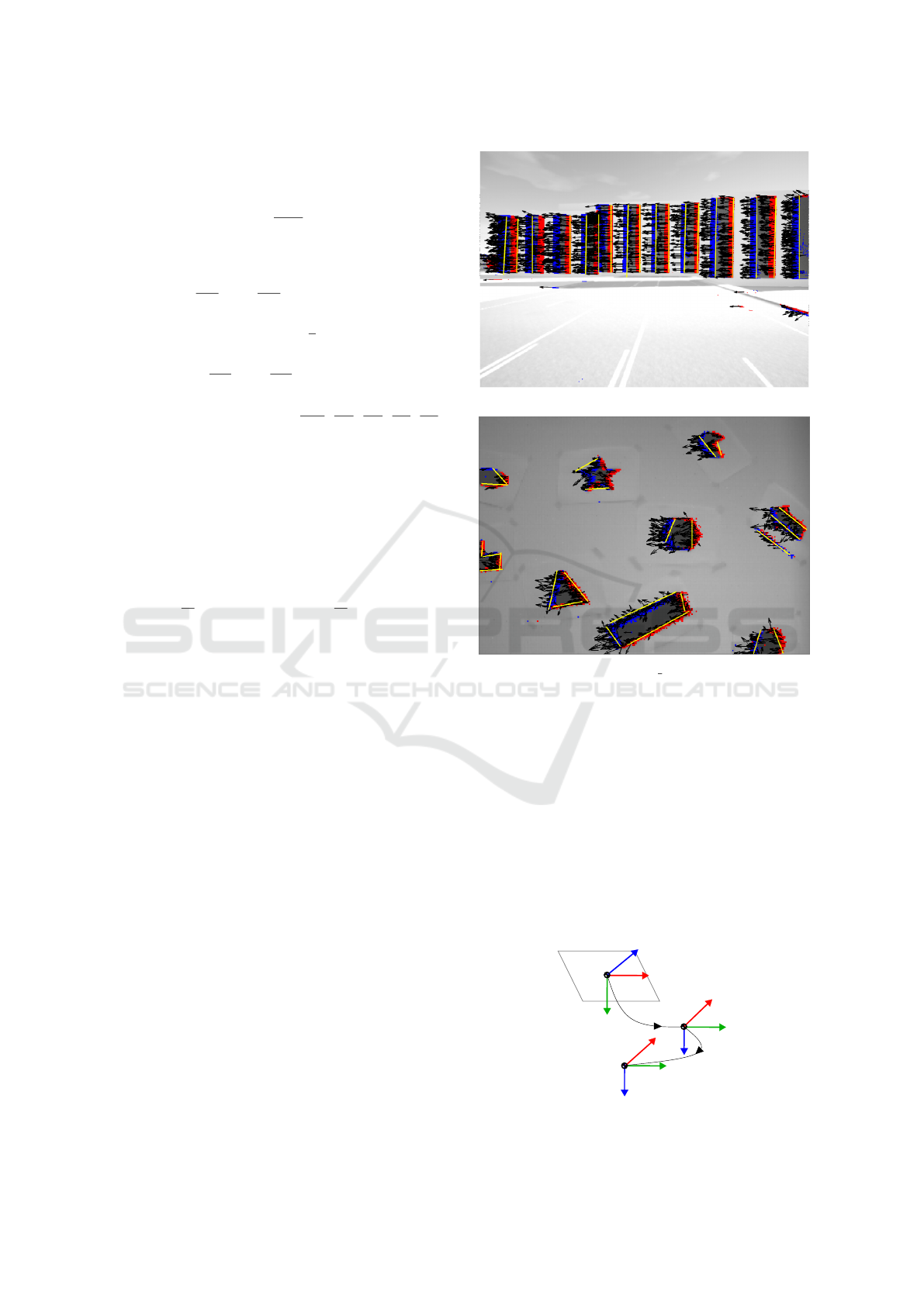
(a) IBISCape sequance.

(b) shapes 6dof.

Figure 4: Grayscale images of the sequences used to test our

algorithm with the triggered events (red for positive polarity

and blue for negative polarity). The estimated optical ﬂow

arrows in black and the detected lines in yellows.

Event-based cameras provide information about

contours and that the lines are one of the repetitive

geometric patterns in the environment. We exploit

the detected lines (Khairallah et al., 2022a) to aug-

ment the prior information we know about the envi-

ronment. We assume that the IMU and the camera are

calibrated with initial camera intrinsic parameters val-

ues and the extrinsic transformation T

between DVS

sensor and IMU (illustrated in Figure 5) is known.

To ensure a reliable online calibration of the camera-

World (W)

IMU (I)

DVS (C)

Figure 5: Event camera reference coordinate frames.

VISAPP 2023 - 18th International Conference on Computer Vision Theory and Applications

968

IMU setup, all the intrinsic and extrinsic parameters

of both the DVS and IMU sensors are considered as

optimization states. To ﬁnd 6-DoF initial pose using

optical ﬂow, we need to know the depth of events and

to estimate depth we need the 6-DoF pose. We iter-

atively estimate an initial depth then use it to correct

for accurate pose and twist estimation.

4.3.1 Initial Depth Estimation

The line detection algorithm provides the line param-

eters (center point, line vector and principal optical

ﬂow) and the assigned events to each line. A 2D pro-

jected line on the image plane may have varying depth

in 3D. However, the depth of events around the line’s

center point presents small depth variations (see Fig-

ure 3). We use the estimated optical ﬂow and the IMU

measurements to estimate the depth according to (5).

Since linear velocity is obtained from single integra-

tion of IMU measurements and the angular velocity is

directly provided, we use a sliding average window to

alleviate the effect of accelerometer white noise with-

out removing the gravity vector offset. Gyroscope an-

gular velocities bias offset and white noise are ﬁltered

out using a band pass ﬁlter. For each set of events

around a line, we use Equation (5) where the only un-

known is the inverse depth so each optical ﬂow gives

two depth values and equation becomes:

= ( ˙x − B(x

)Ω)/(A(x

) (25)

where the division here is element-wise division. The

depth ratio





should be identity because they

belong to the same event. If the depth ratio is not in

a bounded interval [th

,th

], this implies that the es-

timated optical ﬂow is highly corrupt and will be re-

jected. The initial depth assigned to all events of the

line is the mean of the estimated depth around the cen-

ter after rejecting outliers. This initialization method

is only effective if the depth does not vary much along

each line, i.e. downward facing cameras of drones or

cameras moving indoor in front of walls.

4.3.2 Initial Pose and Twist Estimation

Using estimated depth of all events around center

point of detected lines and after rejecting outlier op-

tical ﬂow, we re-inject the depth values into Equation

(5) after modifying it so that it becomes (for a single

event):











− f

−c

)

.. .

−c

)(y

−c

)

−



f +

−c

)



− c

)

− f

−c

)

.. .



f +

−c

)



−

−c

)(y

−c

)

−(x

− c

)







∨

˙x

= C(x

)ζ

∨

(26)

In Equation (26), the twist vector ζ

∨

is the only un-

known. We can stack the optical ﬂow information for

all events as:







)







∨







˙x







. (27)

Equation (27) can be solved for ζ

∨

using least square

method for Ax = b where the solution would be

−1

b. Estimating the depth and twist is re-

peated iteratively until convergence to make sure ini-

tialized depth and twist are correctly estimated. The

initial pose is estimated by integrating the twist vec-

tor.

5 EXPERIMENTAL SETUP

Our proposed visual-inertial odometry scheme per-

forms in structured environments containing lines

with low depth variations. For this purpose, we

choose sequences fulﬁlling these criteria in order to

provide a fair assessment. We used one of IBISCape

sequences provided in (Soliman et al., 2022) of a

car moving in an environment augmented with white

walls and black rectangles at different depths. Addi-

tionally, we used the sequence of shapes 6dof pro-

vided in (Mueggler et al., 2017) of a handheld cam-

era moving randomly in front of different geomet-

ric shapes depicted on a wall. These sequence were,

ﬁrst, passed through the optical ﬂow estimator then

the lines detector to have all the required information

for optimization (see Figure 4).

We use Ceres solver (Agarwal et al., 2022) as an

optimizer for its automatic differentiation capability.

Our algorithm run on a 3GHz Core i7 16 core Linux

machine. We have set our time step to 0.025 s where 5

IMU measurements are preintegrated for IBISCape’s

sequence and 25 measurements are preintegrated for

Table 1: Speciﬁcations of the used sequences.

Sequence events Total IMU V

max

Ω

max

[Mevent] Time [s] [Hz] [m/s] [

◦

/s]

IBISCape 21.65 17.6 200 Hz 7.7 76

shape 6dof 17.96 59.7 1000 Hz 2.3 715

Flow-Based Visual-Inertial Odometry for Neuromorphic Vision Sensors Using non-Linear Optimization with Online Calibration

969

Table 2: Detailed quantitative analysis based-on the Average Root Mean Square Error metric of IBISCape and shapes 6dof

sequence. We report results for 25, 50, and 75 percent of dropped events as milestones for brevity.

Method

IBISCape sequence shapes 6dof sequence

µ [m] σ [m] µ [

◦

] σ [

◦

] µ [m] σ [m] µ [

◦

] σ [

◦

]

EVO (Rebecq et al., 2017a) 0.1369 0.0082 1.7840 0.6214 0.09103 0.0051 5.0217 0.9851

Proposed (All events) 0.1204 0.0079 1.5602 0.7683 0.0802 0.0043 2.5791 1.9732

Proposed (25% dropped) 0.1231 0.0117 1.5874 0.8024 0.0841 0.0094 2.8041 1.8541

Proposed (50% dropped) 0.1217 0.0172 1.4272 0.8401 0.0971 0.0158 2.8460 1.9471

Proposed (75% dropped) – – – – – – – –

Table 3: Ablation study on the event-based VI system architecture. We report the mean position errors as a percentage of the

sequence total distance [%].

Method

shapes poster dynamic

6dof translation 6dof translation 6dof translation

IDOL (Le Gentil et al., 2020) 10.4 10.2 12.4 14.0 10.8 5.0

EVIO (Zihao Zhu et al., 2017) 2.69 2.42 3.56 0.94 4.07 1.90

Rebecq et al. (Rebecq et al., 2017b) 0.42 0.50 0.40 0.46 0.56 0.39

(E + I) (Vidal et al., 2018) 0.48 0.41 0.30 0.15 0.38 0.59

Proposed (All events) 0.41 0.45 0.33 0.11 0.17 0.81

Table 4: Study on the effect of events dropping percentage

on the total optimization time reported for the shapes 6dof

sequence.

drop packet packet residual and linear Total

[%] size [−] time [s] jacobian solver [s] time [s]

time [s]

– 50 0.25 0.420759 0.304085 0.724844

– 100 0.5 0.624733 0.496576 1.121309

– 150 0.75 0.956266 0.912470 1.868736

– 200 1 1.059416 0.998935 2.058351

25 50 0.25 0.262560 0.091245 0.353805

25 100 0.5 0.545977 0.215199 0.761176

25 150 0.75 0.729159 0.275548 1.004707

25 200 1 0.845035 0.317980 1.163015

50 50 0.25 0.235112 0.082975 0.318087

50 100 0.5 0.345446 0.104557 0.450003

50 150 0.75 0.465738 0.133461 0.599199

50 200 1 0.627081 0.188407 0.815488

75 50 0.25 0.691566 0.113761 0.805327

75 100 0.5 0.997071 0.208451 1.205522

75 150 0.75 1.285245 0.418131 1.703376

75 200 1 1.375911 0.537240 1.913151

the shapes 6dof sequence. Being recorded with a

handheld camera, shapes 6dof sequence undergoes

high rotational speed and relatively low translational

speed while IBISCape’s sequence have the opposite

characteristics since it’s recorded as a car’s onboard

camera.

6 RESULTS

IBISCape’s sequence had a higher RMSE for trans-

lation because of its high translational speed. In con-

trast, shapes 6dof sequence attained a lower RMSE

for translation for the same reason. The rotational

RMSE error is maintained relatively small because

of the accuracy of the IMU measurements. Figure 7

shows the translational and rotational errors over time

for the two line-based feasible applications. The ﬁrst

is the vehicle moving in a line staged textured road

(IBISCape sequence), where the errors are reported

in terms of 10’s of [cm]. Whereas, the second ap-

plication of a handheld DAVIS sensor facing shapes

with clear lines, where the errors are reported in terms

of 10’s of [mm]. However, both sequences show a

high standard deviation for the rotational errors re-

sults from the low accuracy in the gyroscope noise

covariance estimation during IMU still calibration.

We ran many experiments to check for the ac-

curacy of our system with and without dropping

events to alleviate for real-time computation. The

assumption that our scheme will still work in case

of events being dropped is made since it only de-

pends on optical ﬂow (and not tracked features) and

that the number of optimization residuals is always

much lower than the amount of events at each time

step. We found that our system can hold accurate re-

sults until we reach around 50% of dropped events

for shapes 6dof sequence and about 60% of dropped

events for IBISCape’s sequence (see Table 2). The

amount of events that can be dropped depends on

events frequency. IBISCape’s sequence maintained

good results while more events were dropped because

of its higher resolution and events’ frequency.

The accuracy did not vary much before failure oc-

curred with 75% events dropping, which validates the

assumption that events can be dropped with a thresh-

old depending on events frequency and camera res-

olution. Dropping the events can also be improved

to maintain accuracy by choosing the dropped events

being assigned to lines where each line should have a

VISAPP 2023 - 18th International Conference on Computer Vision Theory and Applications

970

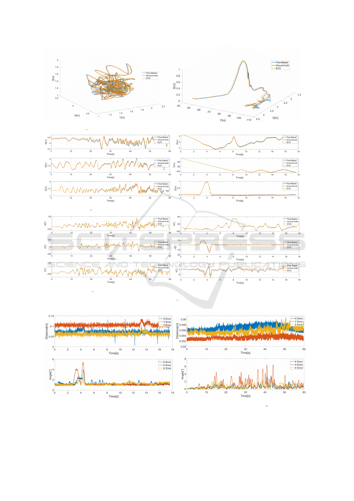
(a) shapes 6dof sequence estimated pose.

(b) IBISCape’s sequence estimated pose.

(d) IBISCape’s position in each axis.

(e) shapes 6dof angles in each axis.

(f) IBISCape’s angles in each axis.

Figure 6: The estimated pose, position and angles of shapes 6dof and IBISCape sequences. Flow-Based method in blue,

the ground truth in red and EVO in yellow.

(a) Position and angle errors of IBISCape sequence. (b) Position and angle errors of shapes 6dof sequence.

Figure 7: Errors of our ﬂow-based visual-inertial odometry method.

Flow-Based Visual-Inertial Odometry for Neuromorphic Vision Sensors Using non-Linear Optimization with Online Calibration

971

Figure 8: On-hardware real-time performance analysis.

minimum amount of events to avoid failure.

To measure the computational time of our scheme,

measurements to be optimized are placed in a sliding

window where previously optimized poses are con-

sidered constant and only the sliding window is opti-

mized. Table 4 shows the computational time of dif-

ferent windows with different percentages of dropped

events. The high computational time for IBISCape’s

sequence is due to the high number of events gener-

ated by a 1024× 1024 camera resolution. On the con-

trary, shapes 6dof sequence attained real-time per-

formance for all the sliding windows with no dropped

events.

The number of IMU measurements and the

amount of events to be dropped deﬁnes the com-

promise to achieve real-time applicability (see Fig-

ure 8). We should keep the smallest possible sliding

window with the maximum amount of events to be

dropped which leads to a trade-off between compu-

tational time and accuracy (sliding windows allowing

real-time performance are shown in bold within Ta-

ble 4). We notice an increase in the computation time

when 75% of the events are dropped as a result of an

abrupt increase in the problem uncertainty due to the

low number of optical ﬂow edges as illustrated in Fig-

ure 2 (b), and hence, low information about the scene.

In Table 3, we represent an ablation study to in-

tellect the contribution of the event-based VI system

conﬁguration on the pose estimation accuracy. The

main conclusion from this quantitative analysis is that

our method outperforms IDOL, an alternative state-

of-the-art line-based method that does not incorporate

optical ﬂow, and can perform well in a line textured

environments.

7 CONCLUSION

We introduce a ﬂow-based visual-inertial odometry

algorithm for neuromorphic vision sensors. The al-

gorithm corrects optical ﬂow information using IMU

measurements in environments where lines can be de-

tected. We run our algorithm without the need for

triangulation or keyframe estimation, which provides

the liberty to choose the size of our sliding window

during optimization.

Instead of running for only scenarios where the

depth of lines does not vary much, the optimal perfor-

mance of our method can be witnessed when backed

with a depth sensor. Integrating a depth sensor can

also be used to estimate more accurate optical ﬂow.

Another improvement to our system would be adding

a place recognition in order to have the ability to close

the loop in a complete SLAM system.

REFERENCES

Agarwal, S., Mierle, K., and Team, T. C. S. (2022). Ceres

Solver.

Baker, S. and Matthews, I. (2004). Lucas-kanade 20 years

on: A unifying framework. International journal of

computer vision, 56(3):221–255.

Censi, A. and Scaramuzza, D. (2014). Low-latency event-

based visual odometry. In 2014 IEEE International

Conference on Robotics and Automation (ICRA),

pages 703–710. IEEE.

Chirikjian, G. S. (2011). Stochastic models, information

theory, and Lie groups, volume 2: Analytic methods

and modern applications, volume 2. Springer Science

& Business Media.

Cyganek, B. and Siebert, J. P. (2011). An introduction to

3D computer vision techniques and algorithms. John

Wiley & Sons.

Forster, C., Carlone, L., Dellaert, F., and Scaramuzza,

D. (2016). On-manifold preintegration for real-

time visual–inertial odometry. IEEE Transactions on

Robotics, 33(1):1–21.

Furgale, P., Barfoot, T. D., and Sibley, G. (2012).

Continuous-time batch estimation using temporal ba-

sis functions. In 2012 IEEE International Confer-

ence on Robotics and Automation, pages 2088–2095.

IEEE.

Gehrig, D., Gehrig, M., Hidalgo-Carrio, J., and Scara-

muzza, D. (2020). Video to events: Recycling video

datasets for event cameras. IEEE Conf. Comput. Vis.

Pattern Recog. (CVPR), pages 3583–3592.

Huber, P. J. (1992). Robust estimation of a location param-

eter. In Breakthroughs in statistics, pages 492–518.

Springer.

Khairallah, M. Z., Bonardi, F., Roussel, D., and Bouchafa,

S. (2022a). Flow-based line detection and segmenta-

tion for neuromorphic vision sensors. In 2022 The

VISAPP 2023 - 18th International Conference on Computer Vision Theory and Applications

972

29th IEEE International Conference on Image Pro-

cessing (IEEE ICPR). IEEE.

Khairallah, M. Z., Bonardi, F., Roussel, D., and Bouchafa,

S. (2022b). Pca event-based optical ﬂow: A fast and

accurate 2d motion estimation. In 2022 The 29th IEEE

International Conference on Image Processing (IEEE

ICIP). IEEE.

Kim, H., Handa, A., Benosman, R., Ieng, S.-H., and Davi-

son, A. J. (2008). Simultaneous mosaicing and track-

ing with an event camera. J. Solid State Circ, 43:566–

576.

Kim, H., Leutenegger, S., and Davison, A. J. (2016). Real-

time 3d reconstruction and 6-dof tracking with an

event camera. In European Conference on Computer

Vision, pages 349–364. Springer.

Kueng, B., Mueggler, E., Gallego, G., and Scaramuzza,

D. (2016). Low-latency visual odometry using event-

based feature tracks. In 2016 IEEE/RSJ International

Conference on Intelligent Robots and Systems (IROS),

pages 16–23. IEEE.

Le Gentil, C., Tschopp, F., Alzugaray, I., Vidal-Calleja, T.,

Siegwart, R., and Nieto, J. (2020). Idol: A framework

for imu-dvs odometry using lines. In 2020 IEEE/RSJ

International Conference on Intelligent Robots and

Systems (IROS), pages 5863–5870. IEEE.

Liu, M.-y., Wang, Y., and Guo, L. (2017). 6-dof motion

estimation using optical ﬂow based on dual cameras.

Journal of Central South University, 24(2):459–466.

Longuet-Higgins, H. C. and Prazdny, K. (1980). The in-

terpretation of a moving retinal image. Proceedings

of the Royal Society of London. Series B. Biological

Sciences, 208(1173):385–397.

Lupton, T. and Sukkarieh, S. (2011). Visual-inertial-aided

navigation for high-dynamic motion in built environ-

ments without initial conditions. IEEE Transactions

on Robotics, 28(1):61–76.

Mueggler, E., Gallego, G., Rebecq, H., and Scaramuzza,

D. (2018). Continuous-time visual-inertial odometry

for event cameras. IEEE Transactions on Robotics,

34(6):1425–1440.

Mueggler, E., Huber, B., and Scaramuzza, D. (2014).

Event-based, 6-dof pose tracking for high-speed ma-

neuvers. In 2014 IEEE/RSJ International Conference

on Intelligent Robots and Systems, pages 2761–2768.

IEEE.

Mueggler, E., Rebecq, H., Gallego, G., Delbruck, T., and

Scaramuzza, D. (2017). The event-camera dataset and

simulator: Event-based data for pose estimation, vi-

sual odometry, and slam. The International Journal of

Robotics Research, 36(2):142–149.

Muglikar, M., Gehrig, M., Gehrig, D., and Scaramuzza, D.

(2021). How to calibrate your event camera. 2021

IEEE/CVF Conference on Computer Vision and Pat-

tern Recognition Workshops (CVPRW), pages 1403–

1409.

Rebecq, H., Gallego, G., Mueggler, E., and Scaramuzza, D.

(2018). EMVS: Event-based multi-view stereo—3D

reconstruction with an event camera in real-time. Int.

J. Comput. Vis., 126:1394–1414.

Rebecq, H., Horstschaefer, T., Gallego, G., and Scara-

muzza, D. (2017a). EVO: A geometric approach to

event-based 6-DOF parallel tracking and mapping in

real time. IEEE Robotics and Automation Letters,

2(2):593–600.

Rebecq, H., Horstschaefer, T., and Scaramuzza, D. (2017b).

Real-time visual-inertial odometry for event cameras

using keyframe-based nonlinear optimization. In

BMVC.

Soliman, A., Bonardi, F., Sidib

e, D., and Bouchafa, S.

(2022). IBISCape: A simulated benchmark for multi-

modal SLAM systems evaluation in large-scale dy-

namic environments. Journal of Intelligent & Robotic

Systems, 106(3):53.

Vidal, A. R., Rebecq, H., Horstschaefer, T., and Scara-

muzza, D. (2018). Ultimate slam? combining events,

images, and imu for robust visual slam in hdr and

high-speed scenarios. IEEE Robotics and Automation

Letters, 3(2):994–1001.

Weikersdorfer, D., Adrian, D. B., Cremers, D., and Con-

radt, J. (2014). Event-based 3d slam with a depth-

augmented dynamic vision sensor. In 2014 IEEE

international conference on robotics and automation

(ICRA), pages 359–364. IEEE.

Weikersdorfer, D. and Conradt, J. (2012). Event-based par-

ticle ﬁltering for robot self-localization. In 2012 IEEE

International Conference on Robotics and Biomimet-

ics (ROBIO), pages 866–870. IEEE.

Weikersdorfer, D., Hoffmann, R., and Conradt, J. (2013).

Simultaneous localization and mapping for event-

based vision systems. In International Conference on

Computer Vision Systems, pages 133–142. Springer.

Zhou, Y., Gallego, G., and Shen, S. (2021). Event-

based stereo visual odometry. IEEE Transactions on

Robotics, 37(5):1433–1450.

Zihao Zhu, A., Atanasov, N., and Daniilidis, K. (2017).

Event-based visual inertial odometry. In Proceedings

of the IEEE Conference on Computer Vision and Pat-

tern Recognition, pages 5391–5399.

Zucchelli, M. (2002). Optical ﬂow based structure from

motion. PhD thesis, Numerisk analys och datalogi.

Zucchelli, M., Santos-Victor, J., and Christensen, H. I.

(2002). Multiple plane segmentation using optical

ﬂow. In BMVC, volume 2, pages 313–322.

Flow-Based Visual-Inertial Odometry for Neuromorphic Vision Sensors Using non-Linear Optimization with Online Calibration

973