Trade-off Clustering Approach for Multivariate Multi-Step Ahead

Time-Series Forecasting

Konstandinos Aiwansedo, Wafa Badreddine and J

ome Bosche

Department of Science, University of Picardy Jules Verne, 33 rue Saint-Leu, Amiens, France

Keywords:

Artiﬁcial Intelligence, Time-Series Forecasting, Neural Networks, Clustering Algorithms, Machine Learning,

Univariate and Multivariate Time Series.

Abstract:

Time-Series forecasting has gained a lot of steam in recent years. With the advent of Big Data, a consid-

erable amount of data is more available across multiple ﬁelds, thus providing an opportunity for processing

historical business-oriented data in an attempt to predict trends, identify changes and inform strategic decision-

making. The abundance of time-series data has prompted the development of state-of-the-art machine learning

algorithms, such as neural networks, capable of forecasting both univariate and multivariate time-series data.

Various time-series forecasting approaches can be implemented when leveraging the potential of deep neu-

ral networks. Determining the upsides and downsides of each approach when presented with univariate or

multivariate time-series data, thus becomes a crucial matter. This evaluation focuses on three forecasting ap-

proaches: a single model forecasting approach (SMFA), a global model forecasting model (GMFA) and a

cluster-based forecasting approach (CBFA). The study highlights the fact that the decision pertaining to the

ﬁnest forecasting approach often is a question of trade-off between accuracy, execution time and dataset size.

In this study, we also compare the performance of 6 deep learning architectures when dealing with both uni-

variate and multivariate time-series datasets for multi-step ahead time-series forecasting, across 6 benchmark

datasets.

1 INTRODUCTION

Large volume of data are daily generated and stored in

capacious databases, in hopes of being exploited later

on (Oussous et al., 2018). These data can be stored

in different formats and structures. A particular type

of data are time-series data. Time-series is a set of

sequential data collected through repeated measure-

ments over time. When a time-series describes a sin-

gle variable, it is referred to as univariate time-series.

For example, in weather forecasting, past recorded

temperature values are used to predict future temper-

atures. On the other hand, when it involves multiple

variables, it is referred to as multivariate time-series.

An example of a multivariate time-series forecasting

is the forecasting of the future price of Bitcoin based

on historical times series of the price itself, as well

as other variables such as volume and date-derived

features. The plethora of time-series data in recent

years has enriched the ﬁeld of Big Data and prompted

the development of machine learning techniques ca-

pable of dealing with the complexity associated with

such data, whether it be for forecasting, classiﬁca-

tion or clustering purposes. Various statistical mod-

els have been proposed over the years, exclusively

designed for univariate time-series forecasting (Box,

1970). The main downside with most classical time-

series models is that they tend to perform poorly on

nonlinear data and are generally more suited for uni-

variate time-series forecasting.

The limitations associated with statistical tech-

niques have motivated the development of machine

learning algorithms, such as, support vector regres-

sion (SVR), decesion trees, XGBoost, AdaBoost and

deep neural network models, among others. Among

all cited algorithms, deep neural networks have man-

aged to draw signiﬁcant attention.

These models are able to ﬁnd temporal structures,

model seasonality and temporal dependencies in se-

quential data. They have gained quite a reputation

these last years and have been implemented across

multiple ﬁelds for resolving numerous problems such

as natural language processing ,image detection and

recognition, stock exchange forecasting, electricity

load forecasting etc.

When dealing with neural networks for time-

Aiwansedo, K., Badreddine, W. and Bosche, J.

Trade-off Clustering Approach for Multivariate Multi-Step Ahead Time-Series Forecasting.

DOI: 10.5220/0011660100003393

In Proceedings of the 15th International Conference on Agents and Artiﬁcial Intelligence (ICAART 2023) - Volume 2, pages 137-148

ISBN: 978-989-758-623-1; ISSN: 2184-433X

 2023 by SCITEPRESS – Science and Technology Publications, Lda. Under CC license (CC BY-NC-ND 4.0)

137

series forecasting, multiple forecasting approaches

present themselves. Instead of using a separate neu-

ral network model to individually forecast each time-

series of a particular dataset or even implementing

a global model for parallel forecasting, a clustering

approach could also be envisaged for this purpose

(Bandara et al., 2020)-(Tadayon and Iwashita, 2020).

This approach consists of implementing time-series

clustering techniques in order to group homogeneous

time-series into subgroups, with the intention of us-

ing as many neural network models for forecasting

as there are subgroups. The clustering approach was

proposed as a means to overcome global models’ ac-

curacy decrease when presented with multiple hetero-

geneous time-series as input.

In this paper, we propose a comparative study

of the three multivariate time-series forecasting ap-

proaches on 6 benchmark time-series datasets. The

ﬁrst approach, denoted as Separate Model Forecasting

Approach (SMFA), involves individually forecasting

each time-series of a dataset with a separate deep

learning model. The second strategy referred to as a

Global Model Forecasting Approach (GMFA), where

cross-series information sharing is exploited by using

a unique and global model to process in parallel, all

time series at once. The third strategy is dubbed as

Cluster-Based Forecasting Approach (CBFA), which

consists of grouping together similar time-series by

implementing clustering algorithms, prior to the fore-

casting phase. To our knowledge, there has not been

any comparative study of these three approaches in

one single study, with the implementation of multiple

state-of-art time-series deep neural networks. In ad-

dition a hybrid neural network model’s performance

(CNN-GRU) is evaluated and compared to that of in-

dividual deep learning models (MLP, RNN, LSTM,

GRU, CNN) with respect to the Weighted Average

Percentage Error Metric (WAPE) and in terms of ex-

ecution time.

This paper is organized as follows: Section 2 men-

tions the related work associated with local, global

and cluster-based forecasting approaches for univari-

ate and multivariate time-series. Section 3 speciﬁes

the proposed forecasting approaches implemented for

this evaluation. Section 4 details the requirements

needed prior to forecasting approaches performance

evaluation and the results of the clustering algorithms’

tuning is also analyzed. Section 5 presents and dis-

cusses results of our forecasting approaches’ perfor-

mance evaluation, whereas Section 6 draws conclu-

sions on the results of our evaluation and points out

what future work should entail.

2 RELATED WORK

In this section, we present the related work pertaining

to three main approaches implemented when dealing

with time-series forecasting, as well as the research

carried out on deep learning architectures for time-

series predictions.

Local Based Technique for Time-Series Forecast-

ing. When aiming to forecast multiple time-series

in a dataset, one’s traditional approach would be to

individually model each time-series present in the

dataset. Such approach is dubbed a local approach

and exploits univariate time-series datasets. In such

regressive cases, a time-series’ future values only de-

pend on its past observations. There has been a lot

a research done on using deep learning models to re-

gressively forecasts univariate time-series. In (Chan-

dra et al., 2021), a performance evaluation of mul-

tiple deep learning models such as long short term

memory (LSTM), recurrent Neural networks (RNNs),

convolutional neural networks (CNNs) and bidirec-

tional LSTM (BiLSTM), is conducted. These mod-

els are implemented on univariate time-series and a

multi-step ahead forecasting scheme is carried out on

benchmark datasets. The study concluded that bidi-

rectional networks and encoder-decoder LSTM out-

competed their rivals in terms of accuracy for both

simulated and real-world time series problems. In

(Papacharalampous et al., 2018), a univariate time-

series forecasting study is presented. In this study,

temperature and precipitation are predicted using both

machine learning (ML) and statistical methods. Prob-

lems associated with univariate time-series forecast-

ing such as, lagged variable selection, hyperparameter

selection and performance comparison between ma-

chine learning and classical algorithms are explored

and dealt with.

Global Based Techniques for Time-Series Fore-

casting. A unique universal function approximator

can also be used for multivariate time-series forecast-

ing. In such scenarios, a unique deep learning model

takes multiple time-series as input at once, processes

them in parallel and outputs predictions for each time-

series of a dataset. In (Montero-Manso and Hynd-

man, 2021), the local and global principles are stud-

ied and both statistical and deep learning models are

implemented on benchmark datasets. According to

this study, as the length of a series increases so does

the complexity of local models, which is not the case

with global models. The authors showed that global

models with an increased complexity outperformed

local state-of-the-art models on most datasets, with

ICAART 2023 - 15th International Conference on Agents and Artiﬁcial Intelligence

138

way fewer parameters. Nonetheless, they argued that

the beneﬁts of one principle over the other depends

on the context. Their ﬁndings underline the necessity

of further research in the ﬁeld of time-series forecast-

ing. In (Sen et al., 2019), a hybrid model is proposed,

capable of thinking globally but acting locally. The

model achieves such a feat by leveraging its convolu-

tion layers, which capture both local and global time-

series properties in a dataset. The proposed model

outperformed its contenders on 4 benchmark datasets.

In (Wan et al., 2019), a novel multivariate tempo-

ral convolutional network is proposed for multivari-

ate time-series forecasting and compared to existing

widely used models for such tasks, such as LSTMs,

CNNs and multivariate attention-based models.

Clustering-Based Techniques for Time-Series

Forecasting. When dealing with multiple time-

series forecasting problems, a number of approaches

have been put forward over the years in an effort to

ameliorate time-series forecasting accuracy. One of

this approach entails a clustering paradigm, whose

advantages have been detailed in (Bandara et al.,

2020), (Pavlidis et al., 2006), (Asadi and Regan,

2020) , (Cherif et al., 2011) and (Mart

ınez-Rego

et al., 2011). In (Bandara et al., 2020) a clustering

approach was evaluated on two different datasets:

CIF2015 and NN5. On the CIF2015 dataset, the

proposed clustering model outperformed the other

models with respect to the speciﬁc evaluation metrics

used in the competition. On the NN5 dataset, a

model based on the clustering method was the best

performing contender in terms of the average rank-

ings, over the evaluated error measures. A similar

clustering method was put forward in (Tadayon

and Iwashita, 2020), where the clustering approach

results indicated overall forecasting improvements in

terms of accuracy and execution time. In (Pavlidis

et al., 2006), the clustering approach was imple-

mented on a ﬁnancial dataset so as to address noise

and non-stationarity. The experimental results were

promising for one-step-ahead forecasting, while

multi-step ahead forecasting being a more difﬁcult

task. In (Sfetsos and Siriopoulos, 2004), a clustering

method was implemented for pattern recognition on

separate datasets.

In this study (Yatish and Swamy, 2020), clusters

were generated by a data analysis oriented cluster

methodology that formed groups with similar linear

relationships of their most common property. There-

after, a pattern recognition scheme was employed for

forecasting. The proposed scheme showed an im-

provement in terms of error over conventional fore-

casting algorithms. In (Stoean et al., 2020), a simi-

lar approach was implemented, where self-organizing

maps, a shape-similarity clustering model was used

to group similar medical data of patients and prior to

implementing a CNN-LSTM model for classiﬁcation.

Deep Learning Architectures. When it comes to

time-series forecasting, one has multiple avenues for

achieving it. Traditionally, statistical methods such as

ARIMA were the default choice. But the shortcom-

ings of such statistical approaches lead to the develop-

ment of neural network architectures. Initially, Feed

Forward Neural Networks (FFNN) were proposed for

time-series forecasting. Nonetheless, these were not

tailor-made architectures for time-series processing as

they did not take into account the sequentiality as-

sociated with time-series data. Later on, sequential

processing oriented architectures were proposed for

time-series data, most notably, recurrent neural net-

works and its variants such as Elman Recurrent Net-

works (ERNNs), Long Short-Term Memory (LSTM)

and Rated Recurrent Units (GRU), tailor-made for

processing sequential data.

In recent years, convolutional neural networks

(CNNs) which were primarily earmarked for image

and audio processing have also earned quite a repu-

tation in the ﬁeld of time series forecasting, as they

are quite adept at extracting spatial and temporal in-

formation in sequential data and are computationally

cheaper than recurrent neural networks.

Hybrid models based on a combination of sta-

tistical and deep learning models have also recently

emerged. In (Zhang et al., 2019) results showed that

the merging of the two models signiﬁcantly resulted

in reduction in the overall forecasting error, with the

hybrid model being able to capture concurrently both

linear and nonlinear patterns in the dataset. Hy-

brid models based solely on combination of machine

learning models have also been widely studied and

democratized. In (Pan et al., 2020), (Yu et al., 2021)

and (Sajjad et al., 2020), a hybrid CNN-GRU model

is utilized for resolving various tasks such as, wa-

ter level prediction, license plate recognition, oil soil

moisture prediction and short-term residential load

forecasting respectively. Despite the success of super-

vised learning, in particular that of recurrent architec-

tures in the ﬁeld of time-series forecasting, other ma-

chine learning branches have also proposed various

models for time-series forecasting, such as, state spate

models in (Franceschi et al., 2020), representation

learning based models in (Rangapuram et al., 2018)

and natural language processing attention-based mod-

els dubbed transformers in (Grigsby et al., 2021).

Trade-off Clustering Approach for Multivariate Multi-Step Ahead Time-Series Forecasting

139

3 PROPOSED FORECASTING

APPROACHES

In this section, we present in detail three forecasting

approaches:

1. Separate Model Forecasting Approach - SMFA

(section 3.1)

2. Global Model Forecasting Approach - GMFA

(section 3.2)

3. Cluster-Based Forecasting Approach - CBFA

(section 3.3)

These approaches propose a multi-step ahead

time-series prediction scheme, by implementing a

Multi Input Multi Output strategy (MIMO). The pur-

pose of this conducted study is to determine the ap-

propriate way of processing multivariate time-series

for forecasting when exploiting various deep learning

neural network architectures and identifying the most

important factors related to each approach in order to

obtain optimal results.

3.1 Separate Model Forecasting

Approach (SMFA)

SMFA is depicted in ﬁgure 1 and is implemented in

(Wang and Jiang, 2015). It involves individually pro-

cessing each time-series of a dataset with a separate

deep learning model. In this scenario, the forecast-

ing results of a particular time-series are solely based

on the historical data of that particular series. This

is a autoregressive process in which a time series is

explained by its past values rather than that of other

time-series variables.

1 : N Time-Series

1 : N Time-Series1:N Neural Networks

Input Dataset

Predicted Output

Figure 1: Separate Model Forecasting Approach (SMFA).

3.2 Global Model Time-Series

Forecasting Approach (GMFA)

GMFA is presented in ﬁgure 2 and is implemented

in (Karunasinghe and Liong, 2006). In this approach,

cross-series information sharing is being exploited, by

using a unique and global model to process in par-

allel, all time-series at once. In this context, cross-

series information sharing becomes an essential and

decisive factor. Indeed, the predictions of a particu-

lar time-series are inﬂuenced not only by its historical

data but also by those of other time-series contained

in the same dataset.

1 : N Time-Series

1:1 Neural Network

Input Dataset

Predicted Output

Figure 2: Global Model Forecasting Approach (GMFA).

3.3 Cluster-Based Time-Series

Forecasting Approach (CBFA)

CBFA approach is presented in ﬁgure 3. This ap-

proach is based on two phases:

1. Clustering phase: In this phase, time-series are

processed in order to determine similarity in such

a way as to partition the dataset into homogeneous

groups, called clusters (Aghabozorgi et al., 2015).

2. Forecasting phase: During this phase, a separate

deep neural network model is implemented for

each cluster previously identiﬁed in the clustering

phase.

1 : N Time-Series

1 : N Time-Series1:M Neural Networks

Input Dataset

Predicted Output

1:M Clusters

Clustering

Figure 3: Cluster-based Model Forecasting Approach

(CBFA).

Time-series clustering techniques have been ex-

tensively resorted to (Tadayon and Iwashita, 2020) as

tools for resolving plenty of challenges such as mo-

tif discovery, clustering, anomaly detection, classiﬁ-

cation, sub-sequence matching, etc., across multiple

ﬁelds, such as, engineering, ﬁnance, health care, busi-

ICAART 2023 - 15th International Conference on Agents and Artiﬁcial Intelligence

140

ness (Liao, 2005).

In the following, we present three main clustering

algorithms that have been referenced in the literature

and will be exploited for the CBFA approach:

1. The Self-Organising-Map (SOM) algorithm is a

particular type of neural networks, which uses

unsupervised learning to perform dimensionality

reduction (Kohonen, 1982) (Aghabozorgi et al.,

2015). It does so by reducing a multidimensional

input space into a two-dimensional map. It can

also be used for clustering time-series features.

Instead of optimization algorithms, such as gra-

dient descent, the SOM algorithm relies on com-

petitive learning during the learning process. It is

considered as a model-based clustering approach

as it uses the trained weights to determine the ap-

propriate clusters (Aghabozorgi et al., 2015)(Rani

and Sikka, 2012). The SOM algorithm’s dimen-

sions (x and y integer values), that is, the number

of input neurons must be speciﬁed prior to imple-

mentation. We determined the x and y parameters

needed for the SOM algorithm by using a method

employed by practitioners in Equation 1. Later

on, these two parameters will be modiﬁed with the

aim of generating multiple clusters (section 4.5).

x = y = round(( Number of series in dataset )

)

(1)

2. The Ordering points to identify the clustering

structure (OPTICS) is a density-based clustering

algorithm, capable of effectively detecting clus-

ters in data of varying density (Ankerst et al.,

1999). It determines neighboring points by lin-

early arranging them in order, in a manner that

the closest points in space become neighbors. It

identiﬁes core samples of high density, generates

clusters from them and it is well suited for large

datasets. The algorithm requires the number of

samples in a neighborhood for a point to be con-

sidered as a core point (min sample) to be spec-

iﬁed before implementation. This parameter will

be varied at a later stage, for the purpose of pro-

ducing various clusters (section 4.5).

3. K-Means is an unsupervised learning algorithm,

intended for unlabeled data, which involves

grouping similar data points within a dataset into

k clusters. This is usually achieved by a proxim-

ity measure, such as the Euclidean distance. Each

cluster is represented by a prototype and is iter-

atively updated by calculating the mean of each

cluster after points have been assigned (Syakur

et al., 2018). Unfortunately, in order to do so

effectively, the number of clusters is required

beforehand, which is usually unknown when it

comes to untagged data. Different techniques in-

cluding the elbow method are often used to ad-

dress this conundrum.

4 FORECASTING APPROACHES

PERFORMANCE EVALUATION

REQUIREMENTS

In this study, six publicly available datasets were used

to compare the three forecasting approaches (sec-

tion 4.1). These approaches were evaluated based

on WAPE and execution time metrics (section 4.2).

To do so, the hardware requirements needed to carry

out this evaluation study are presented in section 4.3

and the neural networks models’ conﬁguration are

presented in section 4.4. In addition, we have fore-

gone further experimentation to determine the opti-

mal clusters for each dataset (section 4.5) for each

clustering algorithms: SOM (section 1), OPTICS

(section 2) and K-Means (section 3).

4.1 Datasets

In this section, we brieﬂy present 6 publicly avail-

able datasets

used for our study in table 1: Exhang-

eRate datasets, NN5, SolarEnergy, Trafﬁc-metr-la,

WikiWebTrafﬁc and Trafﬁc-perms-bay datasets. These

datasets, originate from different areas, vary from

small to large datasets, with a number of time-series

ranging from 8 to 997 and with the series’ length rang-

ing from 735 to 52105 samples. These datasets have

been used in forecasting competitions and other time

series forecasting reviews such as (Lara-Ben

ıtez et al.,

2021) and (Hewamalage et al., 2021).

Table 1: Six different datasets used in the evaluation of fore-

casting approaches’ performance.

Datasets N of Time-Series Length Source

ExchangeRate 8 7588 Exchange rate data

NN5 111 735 Financial transaction data

SolarEnergy 137 22744 Solar production records

Trafﬁc-metr-la 207 34260 Trafﬁc speed data

WikiWebTrafﬁc 997 550 Wikipedia trafﬁc ﬂow

Trafﬁc-perms-bay 325 52104 Trafﬁc network data

4.2 Evaluation Metrics

To evaluate our three forecasting approaches, we use

the WAPE metric (section 4.2.1) to assess the accu-

racy of predictions as well as completion time (section

Datasets are available at the reviewers’ request

Trade-off Clustering Approach for Multivariate Multi-Step Ahead Time-Series Forecasting

141

4.2.2) to evaluate execution time, which considered a

crucial factor in multiple practical applications. The

Mean Absolute Error (MAE) metric was also used to

evaluate accuracy but was excluded from the study

due to its results being similar to that of the WAPE

metric.

4.2.1 Weighted Average Percentage Error

Metric (WAPE)

The WAPE metric, Equation 2, is a well-known error-

scaling metric when dealing with time series forecast-

ing. It is suited for low volume data and allows com-

parable evaluation across time series of inconsistent

scales (Lara-Ben

ıtez et al., 2021).

WAPE =

∑

i=1

− ˆy

∑

i=1

(2)

where n and i represents the number of observations

and the current observation respectively, y

represents

the actual value of the series and ˆy

represents the pre-

dicted value.

4.2.2 Execution Time

The execution time is considered a crucial evalua-

tion metric. It is used for evaluating the forecasting

approaches’ completion time as well as the execu-

tion time associated with each neural network model.

It also provides variable indications for both fore-

casting approaches and neural models’ performance.

Hence, in the evaluation result section (5.2.2), we will

present:

1. Execution time per forecasting approach: It cor-

responds to the completion time across all imple-

mented neural networks models for each forecast-

ing approach and for each dataset.

2. Execution time per neural network model: It cor-

responds to the completion time of each speciﬁc

neural network model across all forecasting ap-

proaches and for each dataset.

4.3 Hardware Requirements

The evaluation of the three forecasting approaches,

across six different neural networks models and six

different datasets, required an adapted hardware for

the experimentation. Hence, for the hardware speci-

ﬁcations, we used our laboratory distributed memory

system

. It is made up of 2320 computing cores, 20

GPUs, corresponding to a computing power of 225

More details regarding our laboratory system and a

link to its website are available at the reviewers’ request.

teraFLOPS, and 19.4 TB of memory and a visualiza-

tion node (1 GPU). The platform also beneﬁts from

3D scanners, humanoid robots and adapted software.

4.4 Deep Neural Networks’ Parameters

Deep learning models’ parameters that were shared

across 6 deep leaning models for this evaluation are

depicted in Table 2. As for the parameters associated

to each model, they are displayed in Table 3.

Table 2: Deep Learning Models’ Shared Parameters.

Parameters Values

Normalisation (ED) Minmax

Optimizer Adam

Batch size 32

N of epochs 100

Learning Rate 0.01

Past History 30 timesteps

Forecast Horizon 20

Forecasting scheme Multi-Input Multi-Output (MIMO)

Table 3: Deep Learning Models’ Hyperparameters.

Models Parameters Values

MLP Hidden Layers [8, 16, 32, 16, 8]

RNN

Layers

Units

Return sequence

32,32

False, True

LSTM

Layers

Units

Return sequence

32,32

False, True

GRU

Layers

Units

Return sequence

32,32

False, True

CNN

Layers

Filters

Pool size

32,32

2, 2

CNN-LSTM

Layers

Filters - Units

Pool size - Return sequence

1 - 2

64 - 200,100

None - False, True

4.5 Towards Optimal Clusters

Generation

Prior to evaluating the clustering approaches’ per-

formance (CBFA), the goal is to process the time-

series in each dataset and group them into homoge-

neous clusters. To do so, three different clustering

algorithms are used: K-Means, OPTICS and SOM.

However, the clustering algorithms’ results tend to

vary when their hyperparameters are tampered with.

Hence, we proceed in two steps:

1. Clusters generation phase : During this phase, we

implement clustering algorithms on each dataset

to generate clusters. We then vary the parameters

of those clustering algorithms, which results in the

ICAART 2023 - 15th International Conference on Agents and Artiﬁcial Intelligence

142

formation of various clusters for each dataset. The

results associated to each clustering algorithm are

presented in Table 4.

2. Clusters selection phase: Following the clustering

generation phase, we determine the best clusters

for each dataset. We do so, by selecting the clus-

ters with the lowest average WAPE error across 6

neural networks models mentioned in 3 for each

dataset. As a result, we determine the appropri-

ate clusters formations (or in another word, the

appropriate parameters for each clustering algo-

rithm) for each dataset. The results are exhibited

in Figure 4.

The procedure and details associated with the

clusters generation phase for the SOM and OPTICS

algorithms are presented in ﬁgure below. As for the

K-Means algorithm a different technique is imple-

mented for identifying the appropriate clusters :

• With the goal of determining the optimal clusters

for the SOM algorithm, we tamper with the di-

mension parameters (x and y) mentioned in equa-

tion 1. We present ﬁve variations of these param-

eters. Each variation results in a different clusters

formation. For example, SOM

is the result of

determining x and y parameters with equation 1,

and then increasing by 2. The lowest number of

clusters proposed varying the SOM algorithm is

equal to 1 and the highest number of clusters is 49

clusters.

• As for the OPTICS algorithm, we vary the mini-

mum sample (min sample) parameter in section 2.

We vary this parameter 4 times, with each modi-

ﬁcation resulting in a new cluster formation. For

example, OPTICS

is the result of changing the

minimum sample parameter to equal 5. The low-

est number of clusters proposed varying the OP-

TICS algorithm is equal to 1 and the highest num-

ber of clusters is 600 clusters.

• As for the K-Means algorithm, we opt for a differ-

ent technique in determining optimal clusters for

each dataset. Indeed, we instead implement the el-

bow method for determining the optimal number

of clusters needed as input to the algorithm. The

elbow technique is a way of heuristically approxi-

mating the optimal number of clusters in a dataset,

for the K-Means algorithm (Marutho et al., 2018).

It consists of generating clusters for a range of val-

ues of K while using a cost function to estimate

each cluster’s error. When plotted on a graph, it

takes the shape of a curved arm. The resulting

curve, resembling an elbow, dictates the idyllic

number of clusters. The number of cluster cor-

responding to the point of inﬂection on the curve

is then considered the optimal number of clus-

ters needed.(Liu and Deng, 2020). Its selection is

more often than not a trade-off between the pos-

sible number of clusters and the cost function’s

estimated error for each cluster.

Datasets

Average WAPE for clusters-only approaches

ExchageRate NN5 SolarEnergy Traffic-metr-la WikiWebTrafficTraffic-perms-bay

0.5

1.5

CBFA.K-Means

CBFA.SOM1

CBFA.SOM2

CBFA.SOM3

CBFA.SOM4

CBFA.SOM5

CBFA.OPTICS1

CBFA.OPTICS2

CBFA.OPTICS3

CBFA.OPTICS4

Figure 4: CBFA Clusters’ Average WAPE Error.

5 FORECASTING APPROACHES

PERFORMANCE EVALUATION

RESULTS

In this section, the experimental results of our eval-

uation study are displayed. We proceed to evalu-

ate our 3 forecasting approaches. The ﬁrst approach

being the individual model approach (SMFA) sec-

tion3.1, the second being the global model approach

(GMFA) detailed in section 3.2 and the third one

being the clustering approach section 3.3, proposed

by CBFA.SOM, CBFA.OPTICS and CBFA.K-Means

algorithms, whose most suitable clusters for each

dataset was determined in section 4.5. The accuracy

of both forecasting approaches and neural networks

models are displayed in section 5.1. In addition, the

completion time for both forecasting approaches and

neural networks models are showed in 5.2. The 200

last points of each dataset were used as the training

set.

The radar plots in 5, display the normalized results

described in 5.1, allowing for the comparison of both

forecasting approaches and models’ performance. For

each plot, the smallest value for the WAPE metric,

corresponding to the best approach, is positioned at

the center of the radar plot. They present the aver-

age results obtained over the 10 predictions that were

carried out by each model for each approach.

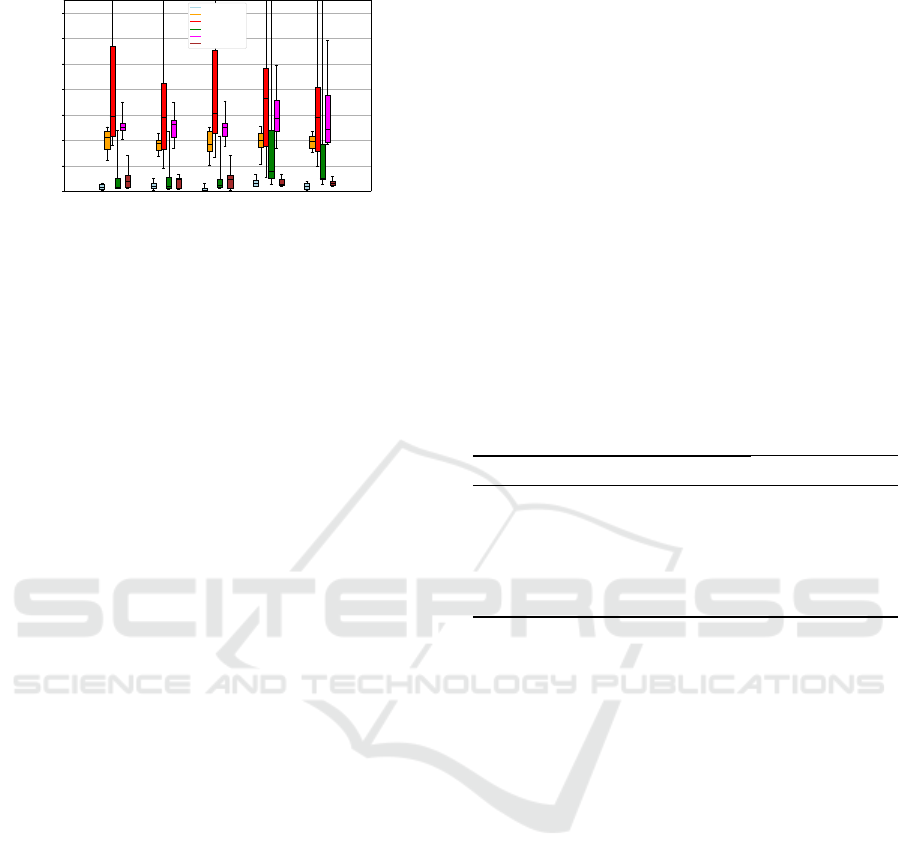
The distribution of the results over the 10 predic-

tions is displayed in ﬁgure 6. This representation al-

lows for a visualization of the average results obtained

per approach and per dataset. The mean value of the

Trade-off Clustering Approach for Multivariate Multi-Step Ahead Time-Series Forecasting

143

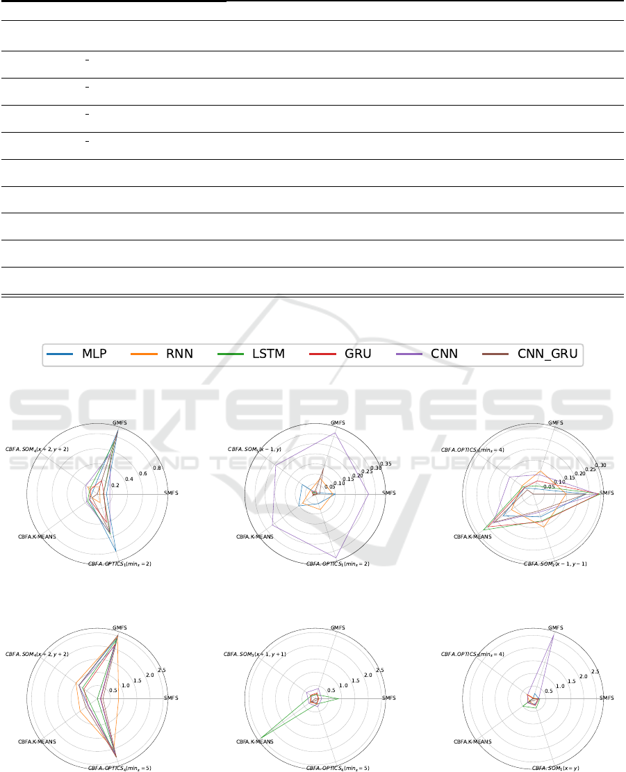
Table 4: Cluster Generation Results.

Clustering Algorithms ExchangeRate NN5 SolarEnergy Trafﬁc-metr-la WikiWebTrafﬁc Trafﬁc-perms-bay

K-means

Execution Time (seconds)

0.11

0.66

3.43

7.06

600

6.04

150

8.57

OPTICS

(min sample=2)

Execution Time (seconds)

0.22

0.09

6.82

24.29

9.05

8.14

OPTICS

(min sample=3)

Execution Time (seconds)

0.01

0.07

0.69

2.23

1.08

7.52

OPTICS

(min sample=4)

Execution Time (seconds)

0.01

0.07

0.68

2.37

1.01

7.58

OPTICS

(min sample=5)

Execution Time (seconds)

0.02

0.06

0.68

2.51

1.15

7.51

SOM

(x = y)

Execution Time (seconds)

93.87

57.44

645.66

1060.82

74.91

6097.14

SOM

(x-1,y-1)

Execution Time (seconds)

33.74

35.87

439.81

57.99

859.35

2866.27

SOM

(x+1,y+1)

Execution Time (seconds)

180.71

67.05

1675.99

87.82

2945.29

8478.53

SOM

(x+2,y+2)

Execution Time (seconds)

301.03

85.86

2719.38

115.82

5529.85

11625.32

SOM

(x-1,y)

Execution Time (seconds)

40.87

40.24

740.79

124.74

1184.59

3820.11

(a) ExchangeRate. (b) NN5. (c) SolarEnergy.

(d) Trafﬁc-metr-la. (e) WikiWebTrafﬁc. (f) Trafﬁc-perms-bay.

Figure 5: Forecasting Approaches’ Evaluation Results.

ICAART 2023 - 15th International Conference on Agents and Artiﬁcial Intelligence

144

SMFA GMFA CBFA.KMEANS CBFA.OPTICS CBFA.SOM

Box Plots For 3 Approaches (6 model s)

0.0

0.2

0.4

0.6

0.8

1.0

1.2

1.4

Average WAPE Error

Box Plots For 3 Approaches (6 models)

ExchangeRate

NN5

SolarEnergy

Traﬃc-metr-la

WikiWebTraﬃc

Traﬃc-perms-bay

Figure 6: Results’ Distribution For 3 Approaches.

WAPE metric is represented by the horizontal bar in

the box plots, the standard deviation by the length of

the boxes, while the minimum and maximum values

are associated with the ends of the segments. This

ﬁgure highlights the effectiveness of the different ap-

proaches, in particular those of the Exchange Rate,

Trafﬁc-metr-la and Trafﬁc-perms-bay datasets, while

showing the variability of the results obtained from

one prediction to another, particularly signiﬁcant for

the Solar Energy dataset.

5.1 Average WAPE Results

For estimating a forecasting approach’s performance

displayed by spider plots in ﬁgure 5, a WAPE er-

ror metric is computed for 6 different neural network

models, i.e., MLP, RNN, LSTM, GRU, CNN, CNN-

GRU, for that particular approach. The overall error

for each forecasting approach is calculated by aver-

aging the the WAPE errors across all neural network

models for each time-series and each dataset.

Table 5 condenses the results of the radar plots de-

picted in ﬁgure 5, by emphasizing this time around

the 2 most advantageous approaches for every dataset

with respect to the WAPE error metric. For the Ex-

changeRate dataset, the individual approach (SMFA)

outperforms other approaches, whereas a variation

of the SOM algorithm (CBFA.SOM

) produces the

second-best results. For the NN5 dataset, a clus-

tering approach (CBFA.SOM

) is the most effective

approach, followed by another clustering approach

CBFA.OPTICS

. As for the solarEnergy dataset,

the most notable approach is the unique approach

(GMFA), which is trailed by a clustering approach

(CBFA.OPTICS

). For the Trafﬁc-metr-la dataset, the

individual approach (SMFA) achieves the best results,

with a clustering approach (CBFA.K-Means) falling

behind it. As for the WekiWebTrafﬁc dataset,the

unique approach (GMFA) claims ﬁrst spot while a

clustering approach (CBFA.OPTICS

) settles for sec-

ond place. At last, as for the Trafﬁc-perms-bay

dataset, a clustering approach (CBFA.OPTICS

) out-

performs other approaches and the unique approach

(GMFA) achieved the second-best results.

In general, the clustering forecasting approaches

(CBFA) perform best on 2 out of 6 datasets (NN5,

Trafﬁc-perms-bay) and maintain second place on 5

out of 6 datasets (ExchangeRate, NN5, SolarEnergy,

Trafﬁc-metr-la and WikiWebTrafﬁc). In other words,

the clustering approaches are either the ﬁrst and the

second-best approach at every instance, in terms of

accuracy. The second-best performing approach tend

to be the SMFA, outdoing other approaches on 2 out

of the 6 datasets (ExchangeRate and Trafﬁc-metr-

la) approach followed by the GMFA approach (So-

larEnergy and WikiWebTrafﬁc). Amongst all clus-

tering approaches, those proposed by the OPTICS

(CBFA.OPTICS) clustering algorithm tend to lead

to better results, followed by those generated by the

SOM and K-Means algorithms respectively.

Table 5: Forecasting Approaches’ Average WAPE Error.

Datasets 1st approach 2nd approach

ExchangeRate SMFA CBFA.SOM

NN5 CBFA.SOM

CBFA.OPTICS

SolarEnergy GMFA CBFA.OPTICS

Trafﬁc-metr-la SMFA CBFA.K-Means

WikiWebTrafﬁc GMFA CBFA.SOM

Trafﬁc-perms-bay CBFA.OPTICS

SMFA

5.1.1 Neural Networks’ Average WAPE Results

Each neural network produces 10 predictions, which

each prediction being of a horizon of 20 samples and

being evaluated by the WAPE metric. In order to es-

timate the overall forecasting performance of a model

on a dataset, the average error across all 10 predic-

tions is computed.

Table 6 summarizes the results portrayed in radar

chart depicted in ﬁgure 5, by highlighting the two

leading neural networks architectures, in terms of av-

erage WAPE error for each dataset. The RNN model

achieves best results on the ExchangeRate dataset. On

the NN5 dataset, the LSTM model beats the other

models and on the Trafﬁc-metr-la dataset, its the GRU

model the comes out on top. Finally, CNN-GRU

model outperforms its competitors on the SolarEn-

ergy, WikiWebTrafﬁc and Trafﬁc-perms-bay datasets.

Overall, the CNN-GRU model performs best on

the 3 largest out 6 datasets (SolarEnergy, WikiWeb-

Trafﬁc and Trafﬁc-perm-bay), with respect to the av-

erage WAPE error metric, which suggest that the

model is more suitable for larger datasets. The model

with the highest average WAPE error consistently re-

mains the CNN model. Moreover, the ﬁndings show

that the CNN model tend to be the worst in at least

Trade-off Clustering Approach for Multivariate Multi-Step Ahead Time-Series Forecasting

145

3 out of 6 datasets (NN5, SolarEnergy and Trafﬁc-

perms-bay). Furthermore, the spider ﬁgures showed

in 5 go to show the sporadic nature of the LSTM

model illustrated on the WikiWebTrafﬁc dataset. In-

deed, although the LSTM model occasionally out-

shines its adversaries, e.g., on the NN5 dataset, it can

substantially become the worst model by a wide mar-

gin e.g., on the WikiWebTrafﬁc dataset, with a WAPE

error 3 times higher (2,44) than the highest observed

CNN-GRU WAPE error (0,77) for the WikiWebTraf-

ﬁc dataset.

Table 6: Neural Network Models’ Average WAPE Error.

Datasets 1st Model 2nd Model

ExchangeRate RNN GRU

NN5 LSTM GRU

SolarEnergy CNN-GRU MLP

Trafﬁc-metr-la GRU CNN

WikiWebTrafﬁc CNN-GRU MLP

Trafﬁc-perms-bay CNN-GRU MLP

5.1.2 Forecasting Approaches and Models’

Lowest WAPE Results

The results obtained for each dataset are described in

the radar ﬁgures 5 . The table 7 summarizes the re-

sults portrayed in radar charts 5, by highlighting the

two leading forecasting approaches and models, in

terms of lowest WAPE error for each dataset. As a

whole, the clustering approaches tend to produce the

ﬁnest results by ranking ﬁrst on 3 out of 6 datasets

(ExchangeRate, NN5, WikiWebTrafﬁc). The SMFA

approach trails the clustering approaches by ranking

second-best on 3 out of 6 datasets (ExchangeRate,

Trafﬁc-metr-la et WikiWebTrafﬁc).The MU approach

also achieves good results by ranking ﬁrst on 2 out

of 6 datasets (SolarEnergy and Trafﬁc-perms-bay).

As far as the neural networks models are concerned,

the results clearly show that the CNN-GRU model

outperforms its rivals by ranking ﬁrst on 5 out of

6 datasets (ExchangeRate, NN5, SolarEnergy, Wiki-

WebTrafﬁc, Trafﬁc-perms-bay). The podium is com-

pleted by the LSTM and GRU neural network models.

Once again, the clustering approaches proposed by

the OPTICS algorithm produce good results on two

datasets (NN5, and WikiWebTrafﬁc).

Table 7: Neural Network Models’ Lowest WAPE Error.

Datasets 1st Model/Approach 2nd Model/Approach

ExchangeRate CNN-GRU-(CBFA.SOM

) RNN (SMFA)

NN5 CNN-GRU (CBFA.OPTICS

) GRU (SMFA.OPTICS

)

SolarEnergy CNN-GRU (MU) MLP (MU)

Trafﬁc-metr-la LSTM (SMFA) CNN (SMFA)

WikiWebTrafﬁc CNN-GRU (CBFA.OPTICS

) GRU (SMFA)

Trafﬁc-perms-bay CNN-GRU (MU) LSTM (MU)

5.2 Completion Time

5.2.1 Forecasting Approaches’ Completion Time

Results

Figure 7 shows the execution time (in hours) per fore-

casting approach presented for our 6 datasets. The

total execution time of an approach is estimated by

summing up the completion time for all 6 neural net-

work models of that approach. As we can observe,

among all approaches , the global model forecasting

approach (GMFA) dominates its rivals by achieving

substantially better results than its opponents, across

all datasets probably due to parallel processing tak-

ing place, making it undoubtedly the dominant choice

when completion time is the most crucial factor. For

example, for the ExchangeRate dataset, the GMFA

approach’s execution time is 0.06 hrs (3.6 minutes),

making it the faster approach for that dataset while the

slowest one is the SMFA approach with an execution

time of 0.55 hrs (32.4 minutes) Another illustrating

example is on the Trafﬁc-perms-bay dataset, where

the GMFA is almost 185 times faster (0.79 hrs) than

the SMFA approach (145.94 hrs). Amongst the clus-

tering approaches, the CBFA. The CBFA.K-Means

approach tends to be the most time-consuming on 4

of the 6 datasets and the CBFA.OPTICS approach ap-

pears to be the least time-consuming clustering ap-

proach. Unsurprisingly, the worst approach in terms

of execution across all datasets is the SMFA approach,

ﬁnishing last at every instance. This is due to the fact

that this approach individually processes each time-

series in a dataset.

5.2.2 Neural Networks’ Completion Time

Results

Figure 8 displays the completion time (in hours) per

neural network model for our 6 datasets. The com-

pletion time for each model is estimated by sum-

ming up the completion time for each model across

all approaches. The results show that CNN-GRU is

the most time-intensive model across all datasets and

conversely MLP has been the least costly neural net-

work model time-wise across all datasets. For exam-

ple, on the Trafﬁc-metr-la dataset, the MLP model

(2.07 hours) is 16 times faster than the CNN-GRU

ICAART 2023 - 15th International Conference on Agents and Artiﬁcial Intelligence

146

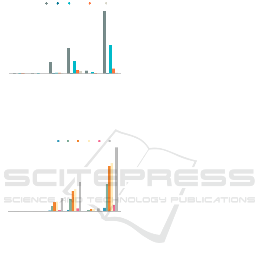
0.54

0.94

26.79

60.35

6.69

145.94

0.06

0.01

0.26

0.44

0.01

0.79

0.27

0.68

1.73

29.47

4.04

67.12

0.54

0.1

1.85

7.47

0.34

11.66

0.07

0.09

1.06

5.39

0.12

2.12

Execution Time (hours)

Datasets

100

120

140

ExchageRate NN5 SolarEnergy Traffic-metr-la WikiWebTraffic Traffic-perms-bay

SMFA GMFA CBFA.KMEANS CBFA.SOM CBFA.OPTICS

Figure 7: Forecasting Approaches’ Average Completion

Time.

model (34.08 hours). The podium is respectively

completed by CNN, RNN, LSTM and GRU neural

network models. The ﬁndings is quite consistent

across all 6 datasets.

0.03

0.08

0.94

2.08

0.57

4.42

0.22

0.27

6.39

14.28

1.63

31.98

0.34

0.41

10.53

23.66

2.4

53.25

0.37

0.44

11.32

25.65

2.61

56.25

0.05

0.09

1.5

3.38

0.62

7.2

0.49

0.57

15.03

34.09

3.4

74.56

Datasets

Execution Time (hours)

ExchageRate NN5 SolarEnergy Traffic-metr-la WikiWebTraffic Traffic-perms-bay

MLP

RNN LSTM GRU CNN CNN_GRU

Figure 8: Deep Neural Networks’ Average Execution Time.

6 CONCLUSION

In this paper, we have conducted a comparative evalu-

ation of 3 time-series forecasting approaches, that is,

the single model forecasting approach (SMFA), the

global model forecasting approach (GMFA) and the

cluster-based forecasting approach (CBFA). To our

knowledge, there has not been any comparative eval-

uation of these three approaches with the implemen-

tation of multiple state-of-art time-series deep neural

networks.

When it comes to determining the best forecast-

ing approach, there is a trade-off to be made between

the three forecasting approaches. The single model

forecasting approach (SMFA) achieves good results

in terms of accuracy but is the most time-consuming

approach. The global model forecasting approach

(GMFA) is the least accurate approach but by far the

most time-saving one. The cluster approach appears

to be a good compromise between SMFA and GMFA,

as it produces good results with respect to the WAPE

metric and is not as time-consuming as the SMFA ap-

proach. The same goes with choosing a neural net-

work model, the neural network model with the best

completion time is the MLP model but the most ac-

curate one is the (CNN-GRU) model which happens

to be the most time-consuming one. Identifying the

appropriate approach and/or model should depend on

the application context, the tasks at hand, the require-

ments and constraints in terms of accuracy and com-

pletion time.

In future work, we intend to enhance our work

by implementing and comparing more recent state-of-

the-art forecasting models, such as, deep state space

models, representation learning models and attention-

based transformers for time-series forecasting. An-

other extension of our work would be to consider

dataset with various time-series lengths instead of

only equal-length time-series. Another interesting

work would be to propose novel time-series forecast-

ing approaches and compare them to current ones.

ACKNOWLEDGEMENTS

We would like to extend our gratitude to the company

Teleric, located in Amiens, France, a major player in

the ﬁeld of connected traceability in the cleaning mar-

ket, that supported our study. We would also like to

thank the Region Hauts-de-France for providing the

resources necessary to carry out this study.

REFERENCES

Aghabozorgi, S., Shirkhorshidi, A. S., and Wah, T. Y.

(2015). Time-series clustering–a decade review. In-

formation Systems, 53:16–38.

Ankerst, M., Breunig, M. M., Kriegel, H.-P., and Sander, J.

(1999). Optics: Ordering points to identify the clus-

tering structure. ACM Sigmod record, 28(2):49–60.

Asadi, R. and Regan, A. C. (2020). A spatio-temporal de-

composition based deep neural network for time series

forecasting. Applied Soft Computing, 87:105963.

Bandara, K., Bergmeir, C., and Smyl, S. (2020). Fore-

casting across time series databases using recurrent

neural networks on groups of similar series: A clus-

tering approach. Expert systems with applications,

140:112896.

Box, G. E. (1970). Gm jenkins time series analysis: Fore-

casting and control. San Francisco, Holdan-Day.

Trade-off Clustering Approach for Multivariate Multi-Step Ahead Time-Series Forecasting

147

Chandra, R., Goyal, S., and Gupta, R. (2021). Evaluation of

deep learning models for multi-step ahead time series

prediction. IEEE Access, 9:83105–83123.

Cherif, A., Cardot, H., and Bon

e, R. (2011). Som time

series clustering and prediction with recurrent neural

networks. Neurocomputing, 74(11):1936–1944.

Franceschi, J.-Y., Dieuleveut, A., and Jaggi, M. (2020). Un-

supervised scalable representation learning for multi-

variate time series.

Grigsby, J., Wang, Z., and Qi, Y. (2021). Long-range

transformers for dynamic spatiotemporal forecasting.

arXiv preprint arXiv:2109.12218.

Hewamalage, H., Bergmeir, C., and Bandara, K. (2021).

Recurrent neural networks for time series forecast-

ing: Current status and future directions. International

Journal of Forecasting, 37(1):388–427.

Karunasinghe, D. S. and Liong, S.-Y. (2006). Chaotic time

series prediction with a global model: Artiﬁcial neural

network. Journal of Hydrology, 323(1-4):92–105.

Kohonen, T. (1982). Self-organized formation of topolog-

ically correct feature maps. Biological cybernetics,

43(1):59–69.

Lara-Ben

ıtez, P., Carranza-Garc

ıa, M., and Riquelme, J. C.

(2021). An experimental review on deep learning ar-

chitectures for time series forecasting. International

journal of neural systems, 31(03):2130001.

Liao, T. W. (2005). Clustering of time series data—a survey.

Pattern recognition, 38(11):1857–1874.

Liu, F. and Deng, Y. (2020). Determine the number of un-

known targets in open world based on elbow method.

IEEE Transactions on Fuzzy Systems, 29(5):986–995.

Mart

ınez-Rego, D., Fontenla-Romero, O., and Alonso-

Betanzos, A. (2011). Efﬁciency of local models en-

sembles for time series prediction. Expert Systems

with Applications, 38(6):6884–6894.

Marutho, D., Handaka, S. H., Wijaya, E., et al. (2018).

The determination of cluster number at k-mean us-

ing elbow method and purity evaluation on headline

news. In 2018 international seminar on applica-

tion for technology of information and communica-

tion, pages 533–538. IEEE.

Montero-Manso, P. and Hyndman, R. J. (2021). Principles

and algorithms for forecasting groups of time series:

Locality and globality. International Journal of Fore-

casting, 37(4):1632–1653.

Oussous, A., Benjelloun, F.-Z., Lahcen, A. A., and Belfkih,

S. (2018). Big data technologies: A survey. Journal

of King Saud University-Computer and Information

Sciences, 30(4):431–448.

Pan, M., Zhou, H., Cao, J., Liu, Y., Hao, J., Li, S., and Chen,

C.-H. (2020). Water level prediction model based on

gru and cnn. Ieee Access, 8:60090–60100.

Papacharalampous, G., Tyralis, H., and Koutsoyiannis, D.

(2018). Univariate time series forecasting of tempera-

ture and precipitation with a focus on machine learn-

ing algorithms: A multiple-case study from greece.

Water resources management, 32(15):5207–5239.

Pavlidis, N. G., Plagianakos, V. P., Tasoulis, D. K., and Vra-

hatis, M. N. (2006). Financial forecasting through

unsupervised clustering and neural networks. Oper-

ational Research, 6(2):103–127.

Rangapuram, S. S., Seeger, M. W., Gasthaus, J., Stella, L.,

Wang, Y., and Januschowski, T. (2018). Deep state

space models for time series forecasting. Advances in

neural information processing systems, 31.

Rani, S. and Sikka, G. (2012). Recent techniques of cluster-

ing of time series data: a survey. International Journal

of Computer Applications, 52(15).

Sajjad, M., Khan, Z. A., Ullah, A., Hussain, T., Ullah, W.,

Lee, M. Y., and Baik, S. W. (2020). A novel cnn-gru-

based hybrid approach for short-term residential load

forecasting. Ieee Access, 8:143759–143768.

Sen, R., Yu, H.-F., and Dhillon, I. S. (2019). Think glob-

ally, act locally: A deep neural network approach to

high-dimensional time series forecasting. Advances

in neural information processing systems, 32.

Sfetsos, A. and Siriopoulos, C. (2004). Time series fore-

casting with a hybrid clustering scheme and pattern

recognition. IEEE Transactions on Systems, Man, and

Cybernetics-Part A: Systems and Humans, 34(3):399–

405.

Stoean, R., Stoean, C., Becerra-Garc

ıa, R., Garc

ıa-

Berm

udez, R., Atencia, M., Garc

ıa-Lagos, F.,

Vel

azquez-P

erez, L., and Joya, G. (2020). A hy-

brid unsupervised—deep learning tandem for elec-

trooculography time series analysis. Plos one,

15(7):e0236401.

Syakur, M., Khotimah, B., Rochman, E., and Satoto, B. D.

(2018). Integration k-means clustering method and

elbow method for identiﬁcation of the best customer

proﬁle cluster. In IOP conference series: materials

science and engineering, volume 336, page 012017.

IOP Publishing.

Tadayon, M. and Iwashita, Y. (2020). A clustering approach

to time series forecasting using neural networks: A

comparative study on distance-based vs. feature-based

clustering methods. arXiv preprint arXiv:2001.09547.

Wan, R., Mei, S., Wang, J., Liu, M., and Yang, F. (2019).

Multivariate temporal convolutional network: A deep

neural networks approach for multivariate time series

forecasting. Electronics, 8(8):876.

Wang, S. and Jiang, J. (2015). Learning natural language

inference with lstm. arXiv preprint arXiv:1512.08849.

Yatish, H. and Swamy, S. (2020). Recent trends in

time series forecasting–a survey. International Re-

search Journal of Engineering and Technology (IR-

JET), 7(04):5623–5628.

Yu, J., Zhang, X., Xu, L., Dong, J., and Zhangzhong, L.

(2021). A hybrid cnn-gru model for predicting soil

moisture in maize root zone. Agricultural Water Man-

agement, 245:106649.

Zhang, Y., Luo, L., Yang, J., Liu, D., Kong, R., and Feng, Y.

(2019). A hybrid arima-svr approach for forecasting

emergency patient ﬂow. Journal of Ambient Intelli-

gence and Humanized Computing, 10(8):3315–3323.

ICAART 2023 - 15th International Conference on Agents and Artiﬁcial Intelligence

148