
Automatic Spine Segmentation in CT Scans
Gabor Revy
a
, Daniel Hadhazi
b
and Gabor Hullam
c
Department of Measurement and Information Systems,
Muegyetem rkp. 3., H-1111 Budapest, Hungary
Keywords:
Spine Segmentation, Image Processing, CT, Dynamic Programming.
Abstract:
The segmentation of the spine can be an essential step in computer-aided diagnosis. Current methods aiming
to handle this problem generally employ an explicit model of some type. However, to create an adequately
robust model, a high amount of properly labeled diverse data is required. This is not always accessible. In this
research, we suggest an explicit model-free algorithm for spine segmentation. Our approach utilizes expert
algorithms that are built on medical expert knowledge to create a spine segmentation from thoracic CT scans.
Our system achieves an IoU (intersection over union) value of 0.7103±0.051 (mean±std) and a DSC (Dice
similarity coefficient) of 0.8295±0.0343 on a subset of the CTSpine1K dataset.
1 INTRODUCTION
Algorithms aiming the higher level of automatization
of computer-aided detection (CADe) and diagnosis
(CADx) systems have been an important area of re-
search in recent decades. These systems can help
to make the detection of lesions and the planning of
medical interventions preventive, more accurate and
faster.
The aim of our research was to create an auto-
matic system to localize and segment the spine on CT
scans of full thoracic field of view. This algorithm
is part of a larger system that segments bones, com-
plemented by the segmentation of the sternum and the
ribs. Based on the segmentation of the rib cage we can
detect several types of lesions or design medical inter-
ventions. Since the whole rib cage is to be segmented,
it is not critical if the segmentation of the spine runs
into the ribs. However, it is important to completely
segment the vertebral body and the spinous process.
There are other applications of spine segmenta-
tion. In the case of image-guided spinal surgery the
main focus is on the spine, therefore the 3D segmenta-
tion is also done differently. The CT scans are created
in a specific way: with a limited field of view and with
the spine in the center. Then the segmentation should
not only consider the spine as a whole, but also dis-
tinguish the individual vertebrae. Therefore, such al-
a
https://orcid.org/0000-0002-4547-3923
b
https://orcid.org/0000-0002-6233-5530
c
https://orcid.org/0000-0002-4765-2351
gorithms must utilize an explicit model. Also, these
algorithms often require manual seed points in order
to function. In our work, however, we aimed to cre-
ate a simple but robust, explicit model-free algorithm
that does not involve manual intervention. Even in
such a simplistic case, there are still many challenges.
First, the varying quality of CT scans can cause diffi-
culties. For example, in some cases the vertebra falls
apart into many small segments of high density with
low-density material in between. Second, the con-
trast agent, which normally facilitates the segmenta-
tion process, complicates the applicability of classi-
cal image processing techniques in this case, as it can
have a high density, similar to bones.
This paper is structured as follows. Section 2 pro-
vides an overview on the relevant previous works.
Section 3 describes the process of the segmentation.
In subsection 3.1 the estimation of the center line of
the spine is described, subsection 3.2 details the cre-
ation of the main segmentation and in subsection 3.3
the refinement of the segmentation mask is detailed.
In section 4 the proposed algorithm is evaluated on
a subset of the publicly available CTSpine1K (Deng
et al., 2021) dataset. The results of our work are sum-
marized in section 5.
The steps of the segmentation algorithm are vi-
sualized using the LIDC-IDRI (Armato et al., 2011)
dataset. The parameters of the proposed algorithms
were also tuned based on this database and expert
knowledge. This dataset contains 1308 thoracic CT
scans of diagnostic and lung cancer screening of 1010
patients.
86
Revy, G., Hadhazi, D. and Hullam, G.
Automatic Spine Segmentation in CT Scans.
DOI: 10.5220/0011660000003414
In Proceedings of the 16th International Joint Conference on Biomedical Engineering Systems and Technologies (BIOSTEC 2023) - Volume 2: BIOIMAGING, pages 86-93
ISBN: 978-989-758-631-6; ISSN: 2184-4305
Copyright
c
2023 by SCITEPRESS – Science and Technology Publications, Lda. Under CC license (CC BY-NC-ND 4.0)

2 RELATED WORK
There are several approaches towards spine segmen-
tation in CT scans. The input can be a CT scan of
full thoracic field of view or the field of view may be
limited to the spine. For some medical procedures it
might be necessary to label the spine at vertebra-level
(multi-class labeling). In other cases, it is sufficient
only to label the spine (binary labeling).
Previously, the segmentation of the spine has
mainly been performed by fitting a shape prior and
deforming it to the actual spine. Athertya et al. used
a set of feature markers from the CT scan to cre-
ate an initial contour for an active contour model
(ACM) (Athertya and Kumar, 2016). This is further
refined by utilizing a fuzzy corner metric, which is
based on the image intensity. Castro-Mateos et al.
utilized a type of statistical shape models, statisti-
cal interspace models (SIMs) to significantly reduce
the overlap between the different vertebrae (Castro-
Mateos et al., 2015). Ibragimov et al. proposed a
multi-energy segmentation framework, which com-
bines landmark detection and shape-based segmenta-
tion (Ibragimov et al., 2017). In their work, landmarks
are used for the non-rigid deformation of their model.
They utilized Laplacian coordinates to find the opti-
mal deformation.
With the emergence of machine learning in image
processing, a significant amount of data-driven learn-
ing algorithms have been proposed. Sekuboyina et al.
utilized two neural networks: one for localisation and
another for segmentation (Sekuboyina et al., 2017).
A 2D attention network provided a low-resolution lo-
calisation of the spine. Then, a 2D-3D U-shaped
network generated high-resolution binary segmenta-
tions. Lessmann et al. proposed an iterative vertebra
segmentation approach utilizing a fully convolutional
network to segment and label vertebrae one after the
other (Lessmann et al., 2019). The network is com-
bined with a memory component in order to retain
information about the vertebrae already segmented.
As it can be seen, most of the algorithms require a
lot of labeled samples to create a model. This is usu-
ally a bottleneck in realization of the methods. Fur-
thermore, the number of manually labeled CT scans
with full thoracic view is limited. Our method is ex-
plicit model-free thus it does not require voxel-level
segmented samples.
3 METHOD
The segmentation pipeline works as follows. First,
(1) a center line of the spine is estimated based on the
Hounsfield unit values using a convolution-based al-
gorithm. From this centerline, the (2) spine is roughly
segmented by utilizing morphological reconstruction.
The (3) boundaries of the resulting segmentation are
truncated based on anatomical prior knowledge. Fi-
nally, the (4) contour of the vertebral body is refined
by a dynamic programming-based parabola fitting al-
gorithm.
3.1 Spine Center Line Estimation
In the first step, a rough bone mask (I
thresh
) is cre-
ated. This is obtained by thresholding the radioden-
sity (Hounsfield unit) values. The effects of different
thresholds were analyzed in a series of experiments,
using CT scans with and without contrast. Based on
these results a threshold value of 150 was selected in
order to ensure, that the bones are extracted even if
the density values are degraded by high amount of
noise. However, this interval overlaps with the density
value of the blood, containing contrast agent. In such
a case, the descending aorta and the heart may also be
segmented and might become merged with the bone
mask. Therefore, in order to avoid such an inclusion,
the segmentation of the descending aorta is subtracted
from the resulting mask. Furthermore, on the axial
slices, the region that is anterior relative to the de-
scending aorta is removed from the mask. In the next
step, the center of the spine is estimated. Among the
sagittal slices the one with the most segmented vox-
els is selected. The index of this slice estimates the
column where the spine is located on the axial slices.
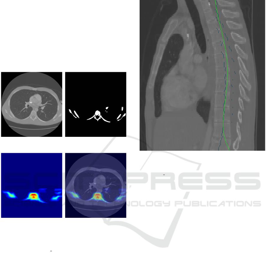
Furthermore, a spine region localization map (M) is
created (see Figure 1), searching for disk-like shapes.
This map is created by convolving the segmentation
(Figure 1b) with the upper (d
u
) and the lower (d
l
) half
of a disk separately and taking the element-wise min-
imum of the results:
d
u
(x, y) = (x
2
+ y
2
≤ r
2
) ∧ (y > 0) (1)
d
l
(x, y) = (x
2
+ y
2
≤ r
2
) ∧ (y < 0) (2)
M = minimum(I
thresh
∗ d
u
, I
thresh
∗ d
l
) (3)
The radius of the disk is set to an average-sized verte-
bra. The motivation of utilizing this type of filtering
is that convolving with a disk shape (i.e. without the
separation of the kernel) resulted in many false posi-
tions due to the contrast agent. This can occur in those
CT image slices, where the mask of the descending
aorta is not present thus the anterior part of the ax-
ial mask cannot be removed. The robustness, in this
case, was further improved by applying the convolu-
tion only to the posterior part of the body (i.e. only to
the lower half of the axial slices). To get an estimated
center line of the vertebrae, in each axial slice of the
Automatic Spine Segmentation in CT Scans
87
filtered image M the point with the highest value is se-
lected. The maximum search is performed in a region
that is defined by the previously estimated column of
the spine center. This search results in a single point
on each slice. Quadratic polynomials are fitted to the
coordinates of the points to filter out outliers. To en-
sure that the fit is robust with respect to outliers, the
RANSAC (Fischler and Bolles, 1981) method is uti-
lized with L1 loss. The projection of the smoothed
center line is shown in Figure 2.
(a) Input CT slice (b) Bone mask created by
thresholding the input CT
(c) Spine region localization
map
(d) Spine region localization
map with overlay
Figure 1: The main steps of the generation of the spine re-
gion localization map for determining a preliminary center
line of the spine. LIDC 0014:50.
3.2 Boundary of the Vertebra
For clarity, the results of the different steps of the al-
gorithm are shown in different colors in Figure 3, and
are referred to in italics in the text. To obtain the
boundary of the vertebra, we start from the bone mask
(red mask) and the center line (green dot C in the mid-
dle) created in the previous step. Several lines are de-
fined, which will determine the bounding region of
the vertebral mask. These lines are defined based on
anatomical prior knowledge approved by medics. To
obtain the end of the spinous process (blue line H3),
maximum intensity projection is performed perpen-
dicular to the sagittal slices followed by thresholding.
This can be computed directly from the bone mask.
Figure 2: Projection of the center line onto a sagittal slice
after polynomial smoothing. Original center points are
marked in blue, whereas the fitted polynomial is the green
line. LIDC 0014.
Since the end of the spinous process is located further
back than the ribs, the bottommost point of the result-
ing segmentation is considered to be the edge of the
spinous process.
In the next step, a basic segmentation mask is
created using morphological reconstruction by dila-
tion (Gonzalez, 2009) with a disk, based on the bone
mask. The seed of the algorithm is created from the
center line, obtained in the previous step. The cen-
ter line only provides a seed region. As long as it
is located within the spine, the morphological recon-
struction applied here can highlight the vertebrae. To
create the seed of the reconstruction the center line
is dilated to ensure that it covers the vertebra. The
algorithm is performed in 2D for each slice. The re-
sulting segmentation mask may overlap with the ribs.
Furthermore, the segmentation may not contain the
spinous process, since it might be detached from the
vertebral body in some slices of the bone mask (as
it can be also seen in Figure 3). This latter prob-
lem was solved by first dilating the resulting mask
across the axial slices (M
R
), intersecting it with the
bone mask (M
B
), and performing a morphological re-
construction with a limited number of iterations using
the result (M
R
∩ M
B
) as the base mask of the recon-
struction. The number of iterations is limited so that
the segmentation does not overlap with nearby struc-
BIOIMAGING 2023 - 10th International Conference on Bioimaging
88
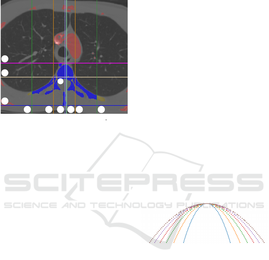
V1 V2
V3
V4
V5 V6
H1
H2
H3
C
Figure 3: Segmentation of the vertebra (LIDC 0014:31).
The bone mask (red+yellowish brown+blue) is created by
thresholding the CT slices. Based on this mask a baseline
spine mask is created (yellowish brown+blue). The colored
lines constrain (yellowish brown → blue mask) the bound-
ing region of the vertebrae by utilizing a priori knowledge.
The magenta and the blue lines denote the top of the ver-
tebra and the end of the spinous process, respectively. The
drab line is drawn to the upper third of the part defined by
these two lines. The width of the baseline spine mask is
marked with the two brown lines. These lines are shifted
both directions with the width resulting in the green lines.
The mint green and purple lines denote the intermediate and
final center line of the spine. The algorithm is detailed in
subsection 3.2.
tures e.g. smaller vessels near the vertebral body. The
obtained segmentation mask is shown in saffron and
blue in Figure 3.
This reconstructed mask is utilized to obtain the
top of the vertebral body (magenta line H1) in the ax-
ial slices. Around the center line, several columns of
the reconstructed mask are selected in a band. In this
band, the upper part of the segmentation is considered
to be the most anterior part of the vertebral body (see
Figure 3).
A more accurate center column (mint green line
V4) of the vertebral body can be determined as fol-
lows. First, the cumulative sum of the number of seg-
mentation pixels is calculated across the columns in
each axial slice. Then, the median of the cumulative
sum determines the center column of the vertebrae.
Using this center column (mint green line V4), the
maximal width (brown lines V2 and V5) of the ver-
tebral body can be determined. This width is used
later to determine the width of the whole vertebra. To
measure the width of the vertebral body in each slice,
the upper third (drab line H2) of the vertebral body is
utilized. This can be derived from the top of the ver-
tebral body and from the end of the spinous process
(blue line H3) calculated earlier.
Separating the ribs from the spine is a difficult
task: there is often no visible sharp line of separa-
tion. To ensure that the mask contains the transverse
process, rather than the ribs, a simple heuristic is uti-
lized: in both directions from the edge of the vertebral
body, the edges are shifted by the width of the verte-
bral body. This approach defines two vertical lines
(green lines V1 and V6), from which the segmenta-
tion is discarded outwards.
After this step, a new, more accurate vertebra cen-
ter column (light purple line V3) can be selected by
utilizing the same algorithm as before.
3.3 Parabola Fitting
The presence of the contrast agent in the blood can
cause non-bony parts to be included in the segmenta-
tion. This means, that small vessels and vessel parts
close to the spine may merge with the spine in the seg-
mentation mask. The anterior part of the vertebrae is
semicircular, which can be segmented more robustly
by curve fitting. Thus we designed a parabola fit-
based correction of the contour of the vertebral body
that utilizes dynamic programming.
First, a family of parabolic curve segments is gen-
erated with the same height and different focal lengths
(see Figure 4). Furthermore, a directional gradient
Figure 4: Family of parabolas that are tested to best fit the
contour of the vertebra.
image is produced from the segmentation mask gen-
erated in the previous step. The gradient image is cal-
culated for each axial slice. Its center is defined by
the final horizontal center and the bottom line of the
upper third of the vertebral body. This gradient im-
age takes a large absolute value with a negative sign
at the upper parabolic border of the vertebral body.
Using exhaustive search, all the parabolas are tested
with different shifts along the y axis. We select the
parabola along which the sum of the gradient values
normalized by the length of the parabola is minimal.
In the next step, the best-fitting parabolas are fit to the
corresponding axial CT slice using dynamic program-
ming (DP). The algorithm is performed separately in
each slice and has two main inputs. The first is the
best-fitting parabola retrieved from the previous step
Automatic Spine Segmentation in CT Scans
89
and sampled at equal distances along the curve. The
second is a directional gradient image produced in the
same way as in the previous step, but this time, it is
based on the input CT slices:
I
dir grad
c
(x) = I
grad
(x)
T
x − c
||(x − c)||
, (4)
where I
dir grad
c
(x) is the gradient image of the CT slice
and c is the centerpoint.
The algorithm can be described by the following
recursion:
T [r, q] =
max
r
′
{T [r
′
, q − 1]−
σ ·
µ
mult
[r] · ||p[q − 1] − c|| − µ
mult
[r
′
] · ||p[q] − c||
}
+ (−1) · I
dir grad
c
(µ
mult
[r
′
] · (p[q] − c) + c), (5)
where p[q] is the q
th
point of the fitted parabola, c is
the center of the parabola, σ is a multiplicative penalty
factor, and µ
mult
[k] is the k
th
multiplication factor that
controls the length of the vector that points from the
center c to the direction of the current point p[q] of the
parabola. Here, T indicates the quality of the multi-
plicative offset r along point q and it is initialized with
zeros: T [row, −1] = 0. As it follows from the recur-
sion, this DP approach tries to balance between align-
ing the contour of the mask to points in the gradient
image that are negative and have a high absolute value
while still maintaining the parabolic shape. In the last
step, the best offset o is selected:
o = argmax
r
′
(T [r
′
, end]), (6)
where ”end” indexes the last point. The ideal offset
for each point of the parabola can then be traced back
from this offset. Based on the points thus fitted, the
segmentation mask can be refined by morphological
reconstruction. Here, the seed mask is the mask under
the fitted points. To create the base mask for the re-
construction, morphological opening is performed on
the segmentation mask above the fitted points. This
ensures, that components linked by only a few pix-
els are detached so that they can be eliminated from
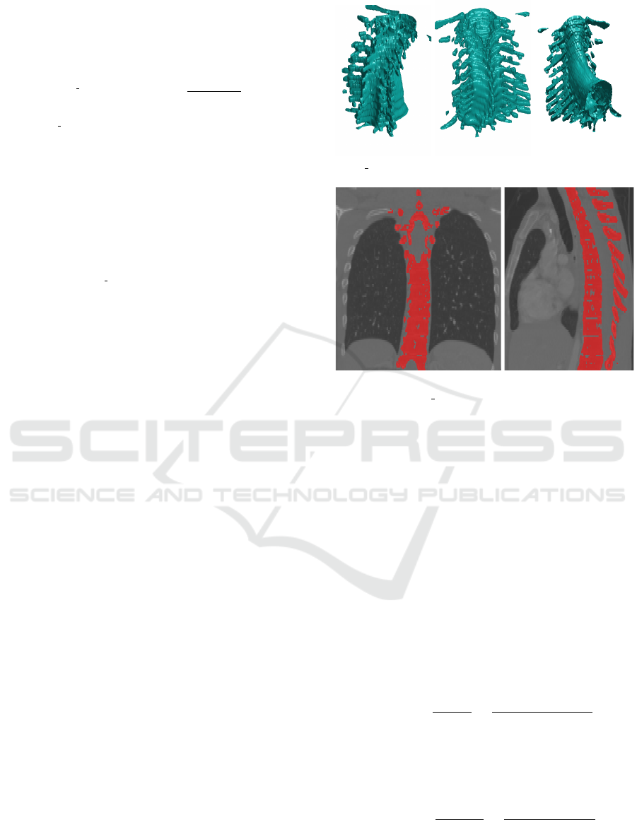
the final segmentation. Figure 7, Figure 8 and Fig-
ure 6 show examples of the results of the algorithm
and Figure 5 shows a full spine segmentation mask in
3D.
4 EVALUATION
Although several spine segmentation datasets were
investigated we chose a dataset that is most relevant
Figure 5: 3D reconstruction of the resulting segmentation.
LIDC 0014.
Figure 6: Coronal and sagittal view of the resulting segmen-
tation on the LIDC 0014 CT scan.
to our target area of application. This means, that the
input CT should be a thoracic CT scan with full tho-
racic field of view. Thus, our proposed spine segmen-
tation method was evaluated on the COVID-19 (An
et al., 2020) (Harmon et al., 2020) subdataset of the
CTSpine1K (Deng et al., 2021) dataset retrieved from
TCIA (Clark et al., 2013a). The COVID-19 dataset
consists of unenhanced chest CT scans from 632 pa-
tients with COVID-19 infections at initial point of
care. 20 of these were selected and manually anno-
tated in the CTSpine1K dataset.
Two evaluation metrics were used for the evalua-
tion of the accuracy of the proposed algorithms. In-
tersection over union (IoU) is the ratio of the intersec-
tion and union of the segmentation mask defined by
the algorithm (A) and the manual labeling (B):
IoU(A, B) =
|A ∩ B|
|A ∪ B|
=
|A ∩ B|
|A| + |B| − |A ∩ B|
(7)
The Dice similarity coefficient (DSC) equals
twice the intersection of the segmentation mask vol-
umes divided by the sum of the volumes:
DSC(A, B) =
2|A ∩ B|
|A| + |B|
=
2|A ∩ B|
|A ∪ B| + |A ∩ B|
(8)
The results of the evaluation are shown in Table 1.
Furthermore, Figure 9 shows the distribution of the
evaluation results.
BIOIMAGING 2023 - 10th International Conference on Bioimaging
90
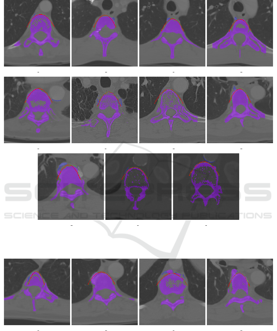
(a) LIDC 0005:81 (b) LIDC 0014:11 (c) LIDC 0014:30 (d) LIDC 0014:32
(e) LIDC 0021:78 (f) LIDC 0022:13 (g) LIDC 0022:65 (h) LIDC 0024:54
(i) LIDC 0024:58 (j) LIDC 0030:106 (k) LIDC 0030:110
Figure 7: Examples, where the dynamic programming-based parabola fitting algorithm improved the spine segmentation. The
best-fitting parabola is colored red and the DP-fitted points are marked in green. The resulting spine segmentation is marked
in purple, while the excluded part is marked in blue.
(a) LIDC 0005:31 (b) LIDC 0018:45 (c) LIDC 0018:92 (d) LIDC 0024:55
Figure 8: Examples, where the dynamic programming-based parabola fitting algorithm did not (fully) improve or worsened
the spine segmentation. The best-fitting parabola is colored red and the DP-fitted points are marked in green. The resulting
spine segmentation is marked in purple, while the excluded part is marked in blue.
The inaccuracy is mainly due to the fact that the
ribs are not completely removed from the segmenta-
tion in cases where they appear to be attached to the
vertebral body in the scan.
Another factor that reduces the measured accuracy
is caused by the inaccuracy of the labeling. Figure 10
Automatic Spine Segmentation in CT Scans
91
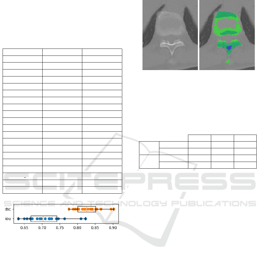
shows an example of this phenomenon. As shown
in the figure, based on the Hounsfield unit values the
ground truth labeling is not complete.
Table 1: Spine segmentation accuracy results on the
COVID-19 (An et al., 2020) subdataset from the CT-
Spine1K (Deng et al., 2021) dataset.
Patient id IoU DSC
A-0003 0.7218 0.8384
A-0011 0.7637 0.8660
A-0013 0.8226 0.9027
A-0014 0.7632 0.8657
A-0016 0.8100 0.8951
A-0025 0.6938 0.8192
A-0046 0.7090 0.8297
A-0070 0.6575 0.7934
A-0073 0.6583 0.7939
A-0090 0.6971 0.8215
A-0096 0.7403 0.8507
A-0106 0.6499 0.7878
A-0120 0.7462 0.8546
A-0147 0.7269 0.8418
A-0154 0.7193 0.8368
A-0173 0.6665 0.7999
A-0187 0.6863 0.8140
A-0202 0 0.6683 0.8012
A-0215 0.6333 0.7755
A-0237 0.6722 0.8040
Figure 9: Spine segmentation accuracy statistics of the eval-
uation: intersection over union (iou) and Dice similarity co-
efficient (dsc).
We also investigated the effect of the parabola
fitting-based refining step. The comparison of the re-
sults is shown in Table 2. This refinement yielded
only a slight improvement: from 0.7086 to 0.7103
and from 0.8284 to 0.8295 in terms of the average IoU
and DSC, respectively. This shows, that in a general
case, it can only slightly improve the segmentation
by removing the segmentation of high-density tissues
close to the vertebral body. This step, however, can
be crucial if a bigger component is still present in the
segmentation due to the morphological reconstruction
step.
For comparison, Deng et al. (Deng et al., 2021)
provide a U-Net (Ronneberger et al., 2015) based
benchmark solution for the CTSpine1K dataset. Their
approach reached a DSC value of 0.985 on the CT-
Figure 10: An example from the evaluation dataset. Blue
denotes the ground truth labeling, whereas the mask created
by the algorithm is marked in green. Based on simply the
Hounsfield unit values, the labeling is not complete.
Table 2: Mean (avg), standard deviation (std) and minimum
(min) of the intersection over union (IoU) and Dice simi-
larity coefficient values from the evaluation results of the
segmentation masks before (baseline) and after (parabola)
applying the parabola fitting-based refinement.
avg std min
IoU
baseline 0.7086 0.051 0.6344
parabola 0.7103 0.051 0.6332
DSC
baseline 0.8284 0.0344 0.7763
parabola 0.8295 0.0343 0.7754
Spine1K and 0.929 on the VerSe dataset (Sekuboy-
ina et al., 2020). However, it is worth noting that the
VerSe database and the majority of the CTSpine1K
database consists of CT scans with a limited field of
view, focusing on the spine. Furthermore, the neural
network based solution provided by Altini et al. (Al-
tini et al., 2021) reached a DSC value of 0.8917 ±
0.0363 on the VerSe dataset.
5 CONCLUSIONS
In this paper we have presented an explicit model-
free segmentation technique for spine segmentation.
The input for the segmentation system is a CT scan
of full thoracic field of view. We have used classical
image processing algorithms and dynamic program-
ming that leverage medical expertise. The advantage
of this approach is that it does not require an explicit
model and is fully automatic. This can be a viable
choice if a fast and simple segmentation is desired
and if it is not critical that the segmentation of the
ribs is not perfectly separated from the spine. How-
ever, in cases where individual segmentation of each
vertebra is required, it is necessary to choose a model-
based solution. A possible limitation of this study
is that the presented method was fine-tuned on the
LIDC-IDRI dataset. Further evaluation on additional
BIOIMAGING 2023 - 10th International Conference on Bioimaging
92

datasets would be preferable, however the availability
of such datasets that contain labeled CT scans of full
thoracic field of view is limited.
ACKNOWLEDGEMENTS
The authors acknowledge the National Cancer Insti-
tute and the Foundation for the National Institutes of
Health, and their critical role in the creation of the free
publicly available (Clark et al., 2013b) LIDC/IDRI
Database (Armato III, Samuel G. et al., 2015) used
in this study; and also the Multi-national NIH Con-
sortium for CT AI in COVID-19. This research was
funded by the National Research, Development, and
Innovation Fund of Hungary under Grant TKP2021-
EGA-02.
REFERENCES
Altini, N., De Giosa, G., Fragasso, N., Coscia, C., Sibi-
lano, E., Prencipe, B., Hussain, S. M., Brunetti, A.,
Buongiorno, D., Guerriero, A., et al. (2021). Segmen-
tation and identification of vertebrae in ct scans using
cnn, k-means clustering and k-nn. In Informatics, vol-
ume 8, page 40. Multidisciplinary Digital Publishing
Institute.
An, P., Xu, S., Harmon, S. A., Turkbey, E. B., Sanford,
T. H., Amalou, A., Kassin, M., Varble, N., Blain,
M., Anderson, V., Patella, F., Carrafiello, G., Turkbey,
B. T., and Wood, B. J. (2020). Ct images in covid-19.
Armato, S., MacMahon, H., Engelmann, R., Roberts, R.,
Starkey, A., Caligiuri, P., McLennan, G., Bidaut,
L., Qing, D., McNitt-Gray, M., et al. (2011). The
lung image database consortium (lidc) and image
database resource initiative (idri): A completed ref-
erence database of lung nodules on ct scans. Medical
Physics, 38(2):915–931.
Armato III, Samuel G., McLennan, G., Bidaut, L., et al.
(2015). Data from lidc-idri.
Athertya, J. S. and Kumar, G. S. (2016). Automatic seg-
mentation of vertebral contours from ct images using
fuzzy corners. Computers in biology and medicine,
72:75–89.
Castro-Mateos, I., Pozo, J. M., Perea
˜
nez, M., Lekadir, K.,
Lazary, A., and Frangi, A. F. (2015). Statistical in-
terspace models (sims): application to robust 3d spine
segmentation. IEEE transactions on medical imaging,
34(8):1663–1675.
Clark, K., Vendt, B., Smith, K., Freymann, J., Kirby, J.,
Koppel, P., Moore, S., Phillips, S., Maffitt, D., Pringle,
M., et al. (2013a). The cancer imaging archive (tcia):
maintaining and operating a public information repos-
itory. Journal of digital imaging, 26(6):1045–1057.
Clark, K., Vendt, B., Smith, K., Freymann, J., Kirby, J.,
Koppel, P., Moore, S., Phillips, S., Maffitt, D., Pringle,
M., Tarbox, L., and Prior, F. (2013b). The cancer
imaging archive (TCIA): Maintaining and operating
a public information repository. Journal of Digital
Imaging, 26(6):1045–1057.
Deng, Y., Wang, C., Hui, Y., Li, Q., Li, J., Luo, S., Sun, M.,
Quan, Q., Yang, S., Hao, Y., et al. (2021). Ctspine1k:
A large-scale dataset for spinal vertebrae segmenta-
tion in computed tomography. arXiv e-prints, pages
arXiv–2105.
Fischler, M. A. and Bolles, R. C. (1981). Random sample
consensus: a paradigm for model fitting with appli-
cations to image analysis and automated cartography.
Communications of the ACM, 24(6):381–395.
Gonzalez, R. (2009). Digital Image Processing. Pearson
Education.
Harmon, S. A., Sanford, T. H., Xu, S., Turkbey, E. B., Roth,
H., Xu, Z., Yang, D., Myronenko, A., Anderson, V.,
Amalou, A., et al. (2020). Artificial intelligence for
the detection of covid-19 pneumonia on chest ct us-
ing multinational datasets. Nature communications,
11(1):1–7.
Ibragimov, B., Korez, R., Likar, B., Pernu
ˇ
s, F., Xing, L.,
and Vrtovec, T. (2017). Segmentation of pathological
structures by landmark-assisted deformable models.
IEEE transactions on medical imaging, 36(7):1457–
1469.
Lessmann, N., Van Ginneken, B., De Jong, P. A., and
I
ˇ
sgum, I. (2019). Iterative fully convolutional neu-
ral networks for automatic vertebra segmentation and
identification. Medical image analysis, 53:142–155.
Ronneberger, O., Fischer, P., and Brox, T. (2015). U-net:
Convolutional networks for biomedical image seg-
mentation. In International Conference on Medical
image computing and computer-assisted intervention,
pages 234–241. Springer.
Sekuboyina, A., Bayat, A., Husseini, M. E., L
¨
offler, M.,
Rempfler, M., Kuka
ˇ
cka, J., Tetteh, G., Valentinitsch,
A., Payer, C., Urschler, M., et al. (2020). Verse: a ver-
tebrae labelling and segmentation benchmark. arXiv.
org e-Print archive.
Sekuboyina, A., Kuka
ˇ
cka, J., Kirschke, J. S., Menze,
B. H., and Valentinitsch, A. (2017). Attention-driven
deep learning for pathological spine segmentation. In
International Workshop on Computational Methods
and Clinical Applications in Musculoskeletal Imag-
ing, pages 108–119. Springer.
Automatic Spine Segmentation in CT Scans
93
