Toward Few Pixel Annotations for 3D Segmentation of Material from

Electron Tomography

Cyril Li

, Christophe Ducottet

, Sylvain Desroziers

and Maxime Moreaud

Universit

e de Lyon, UJM-Saint-Etienne, CNRS, IOGS, Laboratoire Hubert Curien UMR5516,

F-42023, Saint-Etienne, France

Manufacture Franc¸aise des Pneumatiques Michelin, 23 Place des Carmes D

echaux, 63000 Clermont-Ferrand, France

IFP Energies Nouvelles, Rond-point de L’

echangeur de Solaize BP 3, 69360 Solaize, France

Keywords:

Neural Network, Electron Tomography, Weakly Annotated Data, U-NET, Contrastive Learning,

Semi-Supervised Training.

Abstract:

Segmentation is a notorious tedious task, especially for 3D volume of material obtained via electron tomogra-

phy. In this paper, we propose a new method for the segmentation of such data with only few partially labeled

slices extracted from the volume. This method handles very restricted training data, and particularly less than

a slice of the volume. Moreover, unlabeled data also contributes to the segmentation. To achieve this, a combi-

nation of self-supervised and contrastive learning methods are used on top of any 2D segmentation backbone.

This method has been evaluated on three real electron tomography volumes.

1 INTRODUCTION

Electron tomography (ET) (Ersen et al., 2007) is a

powerful characterization technique for the recon-

struction of 3D nanoscale microstructure of material.

Volumes are reconstructed from sets of projections

from different angles acquired by a Transmission

Electron Microscope (TEM) providing a real three-

dimensional information at the nanometric scale. The

limited number of projections and the difﬁculty to

align them correctly (Frank, 2008) produce noisy data

with strong reconstruction artifacts (Figure 1). Stan-

dard segmentation approaches generally fail to pro-

duce accurate semantic segmentation of this kind of

data (Evin et al., 2021), or need intensive expertise of

the user (Fernandez, 2012; He et al., 2008; Volkmann,

2010).

Recently, deep learning (DL) based methods have

been successfully used in this ﬁeld (Akers et al., 2021;

Khadangi et al., 2021; Genc et al., 2022), inheriting

from progresses in 2D or 3D image semantic segmen-

tation (Ronneberger et al., 2015; C¸ ic¸ek et al., 2016;

Milletari et al., 2016; Chen et al., 2018a; Sun et al.,

2019). The standard setup is ﬁrst to train a DL model

on a fully labeled dataset, and then use this model on

the data at hand. However, this approach requires the

availability of a fully segmented set of 3D volumes,

which is a tedious preliminary task. In this paper,

we consider a more realistic semi supervised setup.

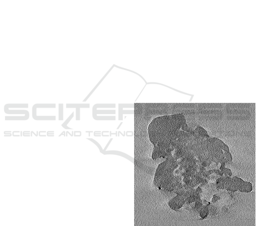
Figure 1: Slice of a volume of zeolite (resolution : 1

nm/voxel). Slices from the volume are noisy and contain

artifacts, that make segmentation tasks harder.

Given a 3D volume, we ask the user to manually seg-

ment only a few regions in a few slices (typically a

single one or two) of this 3D volume. This small

amount of annotated data is then used to train a DL

model, subsequently used to segment the whole 3D

volume.

124

Li, C., Ducottet, C., Desroziers, S. and Moreaud, M.

Toward Few Pixel Annotations for 3D Segmentation of Material from Electron Tomography.

DOI: 10.5220/0011658500003417

In Proceedings of the 18th International Joint Conference on Computer Vision, Imaging and Computer Graphics Theory and Applications (VISIGRAPP 2023) - Volume 5: VISAPP, pages

124-131

ISBN: 978-989-758-634-7; ISSN: 2184-4321

 2023 by SCITEPRESS – Science and Technology Publications, Lda. Under CC license (CC BY-NC-ND 4.0)

The problem of few available training data is not

speciﬁc to ET and has been addressed in many com-

puter vision tasks, mainly using transfer learning (Pan

and Yang, 2009; Wurm et al., 2019). A promising ap-

proach is to rely on contrastive representation learn-

ing, whose goal is to learn an embedding space using

pairs of positive or negative samples (Hadsell et al.,

2006; Dosovitskiy et al., 2014; Zhao et al., 2021). In a

supervised setting, mainly used in Siamese networks

(Koch et al., 2015), positive pairs are taken from sam-

ples of the same class and negative ones are taken

from samples of different classes. The unsupervised

setting relies on positive pairs obtained from a single

sample subject to two independent random perturba-

tions. It was shown to be a powerful self-supervised

learning method (Chen et al., 2020; Chen and He,

2021).

In this article, we propose a new semi-supervised

approach to segment a full volume in ET with only

few annotated pixels. Our approach fully exploits the

labeled as well as the unlabeled pixels of the partially

annotated slices to learn a speciﬁc pixel-level embed-

ding space relevant for segmentation. More precisely,

given a DL model for semantic segmentation, we ﬁrst

reshape the output to deﬁne a pixel-level embedding

space of dimension D. Then, for training, we rely

on contrastive learning and both a weakly-supervised

stream for labeled pixels and a self-supervised stream

for unlabeled ones (Figure 2). Supervised and self-

supervised contrastive learning are used together to

fully exploit partially-labeled data (Figure 3). The

ﬁnal segmentation is obtained through a pixel-wise

classiﬁcation layer operating in the embedding space

of dimension D.

Our principal contributions are:

• A new semi-supervised learning method for prac-

tical 3D image segmentation in ET, which takes

advantage of contrastive learning and self learning

principles to provide accurate volume segmenta-

tion using only few labeled regions of one or two

speciﬁc 2D slices.

• The model can be easily built on top of any 2D

segmentation DL model.

• We provide detailed experimentation on several

real ET data, and we show that an accurate seg-

mentation is possible with only one slice and 6%

of annotated pixels in this slice.

2 RELATED WORKS

Electron Tomography Segmentation. Due to low

SNR and reconstruction artifacts, segmentation of to-

mograms is a difﬁcult task and manual segmentation

still remains the prevalent method (Fernandez, 2012)

often used in interaction with the user through visu-

alization tools (He et al., 2008), sometimes combined

with various image processing methods as watershed

transform (Volkmann, 2010). Following the promis-

ing development of DL in general semantic segmen-

tation tasks (Ronneberger et al., 2015; C¸ ic¸ek et al.,

2016; Milletari et al., 2016; Chen et al., 2018a; Sun

et al., 2019) some recent works have investigated DL

based techniques in 2D electron microscopy (Akers

et al., 2021; Khadangi et al., 2021). In these works,

the bottleneck of the availability of labeled training

data is addressed either by a semi-supervised few-

shot approach (Akers et al., 2021) or by a scalable

DL model, which requires only small- and medium-

sized ground-truth datasets (Khadangi et al., 2021).

In 3D, we only found a ﬁrst investigation of U-Net

model to multi-class semantic segmentation of a γ-

alumina/Pt catalytic material in a class imbalance sit-

uation (Genc et al., 2022). In this work, 30 labeled

slices and data augmentation are needed to train the

model. To the best of our knowledge, our method is

the ﬁrst one providing accurate 3D segmentation with

only few annotated pixels in a single slice.

Contrastive Learning. Contrastive learning aims to

exploit labels better, usually with Siamese networks

(Zhao et al., 2021). The goal is to construct a la-

tent space in which objects with the same label are

close to each other, and objects with different labels

are far from each other. Positive and negative pairs are

formed. Positive pairs are composed of two objects of

the same class, whereas negative ones are composed

of two objects of different classes. A contrastive loss

function is used during training to bring positive pairs

together and negative pairs far from each other. Con-

trastive learning has shown excellent results in image

classiﬁcation (Chen et al., 2020; Grill et al., 2020;

Khosla et al., 2020; Chen and He, 2021). For se-

mantic segmentation, pairs of pixels can be consid-

ered, and these methods can also train a model with-

out labeled data (Chaitanya et al., 2020). When pairs

are created without the knowledge of the class, only

positive ones can be created. Input images are trans-

formed, and the transformed pixels are compared to

their original version. The images, even transformed,

represent the same object and a similarity function

can be minimized during training.

Semi-Supervised Methods in Semantic Segmenta-

tion. The goal of semi-supervised methods in seman-

tic segmentation is to optimize how labeled and unla-

beled data are exploited together to learn a segmen-

tation task. Transformations can be used in Siamese

network to mix a self-supervised loss with a standard

Toward Few Pixel Annotations for 3D Segmentation of Material from Electron Tomography

125

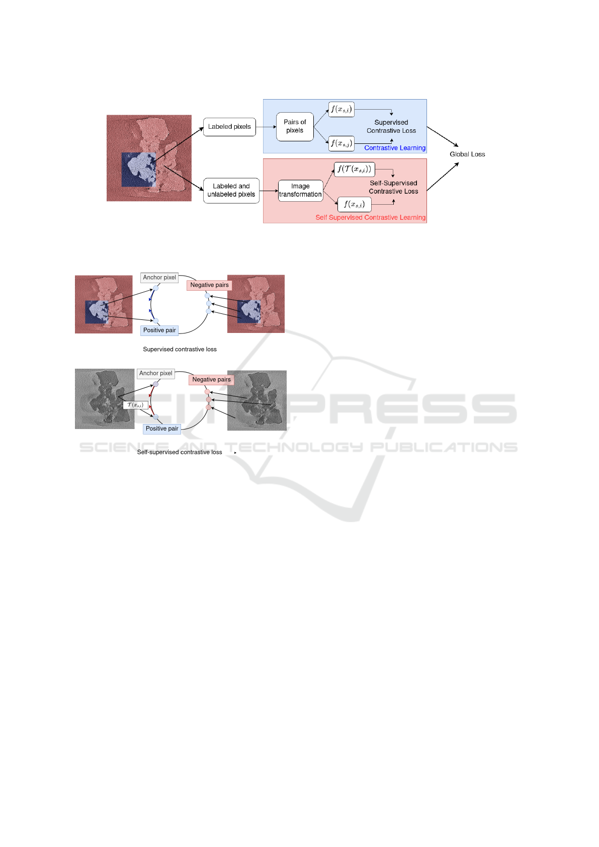
Figure 2: The loss calculation is different depending on pixel labeling. For labeled pixels, pairs of pixels are constructed and

are used in a contrastive loss. For labeled and unlabeled pixels, the training image and the transformed version of itself are

used as a positive pair in a self-learning contrastive loss. Both contrastive loss and similarity loss are added for the global loss.

Figure 3: The supervised contrastive loss is computed for

each labeled pixels. Given a labeled pixel considered as

an anchor pixel, pixels of the same class as this anchor

pixel (positive pairs) are pushed together, while pixels of

a different class (negative pairs) are pushed aside. The self-

supervised loss is computed for both labeled and unlabeled

classes. Given an anchor pixel, a single positive pair is ob-

tained by applying a transform to it, while negative pairs

are obtained from all other pixels. The anchor pixel and its

transformed version are pushed together, while other pixels

are pushed aside from the anchor pixel.

supervised methods (Li et al., 2018). Another ap-

proach is to apply an adversarial method, where two

networks are trained on labeled images. Unlabeled

images are fed into both networks and a similarity

function is minimized (Peng et al., 2020). In (Ouali

et al., 2020), a standard encoder-decoder is used on la-

beled images. Unlabeled images are fed into several

decoders, a slightly modiﬁed version of the decoder

used for the labeled data. The output of all the de-

coders is then compared to the output of the main de-

coder. In this case, the network is transformed. How-

ever, these methods have all their images either fully

labeled or fully unlabeled. In our case, images them-

selves can have unlabeled pixels.

3 PROPOSED METHOD

Our method relies on a 2D representation model

trained with contrastive-learning and self-learning

principles. This model is used to segment each slice

of the volume to provide the ﬁnal 3D segmentation.

Indeed, although several fully 3D convolutional neu-

ral networks (CNN) have been proposed (Milletari

et al., 2016), they were shown to be more resource in-

tensive than 2D models without providing convincing

gains (Kern et al., 2021). The overview of the method

is summarized in Figure 2. The whole architecture

is composed of an encoder-decoder f used to project

pixels of the slice in a pixel level embedding space

and a classiﬁcation layer (a linear model classiﬁer) h

providing the semantic segmentation. The represen-

tation model f is trained using positive and negative

pairs of labeled pixels in the contrastive path, and pos-

itive pairs of labeled and unlabeled pixels in the self-

supervised path. Note that there is a single embedding

space for both labeled and unlabeled pixels. The clas-

siﬁcation layer is subsequently trained using labeled

pixels after freezing the representation model. A stan-

dard weighted cross-entropy loss is used to train this

classiﬁcation layer.

3.1 Formalization

The input volume V is a set of S slices {X

}

s=1,...S

such that each slice X

∈ R

W ×H×1

where W is its

width, H its height and 1 is because the slice is a

grayscale image. We denote x

s,i

the graylevel at pixel

i ∈ I of slice X

, I being the image spatial support.

We then have X

= (x

s,i

)

i∈I

. Each slice is processed

independently. The output segmentation of slice s is

VISAPP 2023 - 18th International Conference on Computer Vision Theory and Applications

126

= h( f (X

)). The encoder-decoder f transforms X

onto Z

= (z

s,i

)

i∈I

= f (X

) ∈ R

W ×H×D

where D is the

dimension of the latent space. The classiﬁcation layer

h performs the pixel-wise class prediction

= h(Z

)

such that

∈ R

W ×H×C

, where C is the number of

classes.

Each voxel of the volume is either labeled or un-

labeled. Let Y

be the pixel-wise class label map of

the slice s, then Y

= (y

s,i

)

i∈I

with y

s,i

∈ {

0, 1, 2, ..., C}

where 1, 2, .., C are the labeled classes and

0 repre-

sents unlabeled pixels. We note L

the set of labeled

pixels and U

the set of unlabeled pixels:

= {i ∈ I , y

s,i

̸=

0}, U

= {i ∈ I , y

s,i

0} (1)

The loss function is computed differently if the

pixel is labeled or unlabeled. Pixels in L

follow the

contrastive path, whereas pixels in L

and U

the self-learning path. For shake of simplicity, in the

following subsections, we will consider the case of a

single labeled slice X

for training, but it can be easily

generalized to any number of training slices by sum-

ming the corresponding losses.

3.2 Contrastive Loss

A contrastive loss is computed for labeled pixels

(Khosla et al., 2020). This loss aims to learn a repre-

sentation space where pixels from the same label are

close to each other in that space, while pixels from

different labels are far from each other in that space.

The contrastive loss is relevant in our case because the

model can be fed with only a few number of labeled

pixels and the contrastive loss can fully exploit each

pixel by forming positive and negative pairs. For each

labeled pixel x

s,i

, i ∈ L

, positive pairs P

s,i

and nega-

tive pairs P

−

s,i

are constructed. As the label is known

for this kind of pixels, given an anchor pixel, posi-

tives pairs are built by choosing pixels of the same

class as this anchor pixel, whereas negatives pairs are

composed of pixels of a different class (Figure 3). We

have:

s,i

= { j ∈ L

, i ̸= j, y

s,i

= y

s, j

} (2)

−

s,i

= { j ∈ L

, i ̸= j, y

s,i

̸= y

s, j

} (3)

Let P

s,i

= P

s,i

∪ P

−

s,i

be the set of pairs that are

formed for each pixel x

s,i

. To balance positive and

negative pairs and limit the computational complex-

ity, we randomly choose an equal number of positive

and negative pairs such that the total number of pairs

per pixel is a given constant value N

The supervised contrastive loss (Khosla et al.,

2020) associated to one labeled slice is deﬁned as:

) =

−1

∑

i∈L

∑

j∈P

s,i

log

exp(sim(z

s,i

, z

s, j

))

∑

k∈P

s,i

exp(sim(z

s,i

, z

s,k

))

(4)

with N

the number of pixels in L

and sim is the

cosine similarity, deﬁned as:

sim(u, v) =

u.v

||u||.||v||

(5)

3.3 Self-Supervised Contrastive Loss

A self-supervised method is used for labeled and un-

labeled pixels. It is especially useful for unlabeled

data, as the information on labels is unknown. To

train without labels, the training slice is transformed,

and a self-supervised contrastive loss is computed be-

tween each transformed image (Chen et al., 2020).

The corresponding pixels, even from slightly trans-

formed images, should have their feature vector close

to each other in the representation space. These two

pixels are considered as a positive pair. All other com-

binations are considered as negative pairs (Figure 3).

Let T be a random transformation of the pixels of the

original slice x

s,i

, i ∈ I. The output Z

of the orig-

inal slice and the output of its transformed version

= f (T (X

)) = (˜z

s,i

)

i∈I

are compared.

The self-supervised contrastive loss associated to

slice X

is deﬁned as:

) =

−1

∑

i∈I

log

exp(sim(z

s,i

, ˜z

s,i

))

∑

j∈I,i̸= j

exp(sim(z

s,i

, z

s, j

))

(6)

where N

is the number of pixels in I.

The ﬁnal loss is a combination of both losses :

L(Z

) = L

) + L

) (7)

4 EXPERIMENTS AND RESULTS

4.1 Implementation Details

For the encoder-decoder f , a U-Net like model is

used to project pixels in the embedding space (Fig-

ure 4). The encoder is composed of three downsam-

pling steps. A downsampling step is composed of two

3 × 3 convolution layers followed by a ReLU layer

and a 2 × 2 Max Pooling layer with a stride 2 for

downsampling. The input image resolution is halved

and the number of channels is doubled for each down-

sampling step. The decoder is also composed of three

steps, with an upsampling layer followed by a 2 ×

Toward Few Pixel Annotations for 3D Segmentation of Material from Electron Tomography

127

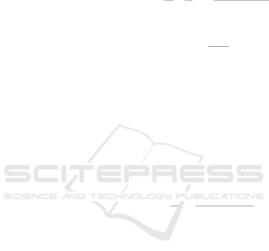
Figure 4: Our model is based on U-Net, with three stages. The output is the projection for each pixel in the embedding space.

A classiﬁcation layer is trained to transform the feature vectors into a segmentation map.

Table 1: Random transformations used to compute the self-

supervised loss.

Transformation Probability Parameters

Gaussian noise 1 N (0, [0.01;0.06])

Gray level shift 0.5 [−0.01;0.01]

Gaussian blur 0.5 σ = [0.5 − 1.5]

2 convolution layer that halves the number of chan-

nels, a concatenation with the corresponding feature

map from the encoder and two 3 x3 convolution lay-

ers followed by a ReLU. As a result, the number of

ﬁlters for each layer of the encoder is 16, 32 and 64.

For each layer of the decoder, the image resolution is

doubled and the number of channels is halved. The

resulting number of layers are 64, 32 and 16. At the

end of the network, a feature map at the size of the

input is obtained. A 1 × 1 convolutional layer is ap-

plied with 16 ﬁlters to project the result in the em-

bedding space. The loss function is computed, de-

pending upon the fact that the pixel is labeled or un-

labeled. To compute the ﬁnal segmentation result, a

pixel-wise classiﬁcation layer h is trained on the out-

put of the training data. This layer is composed of a

single convolutional layer with a kernel of size 1 ×

1. The classiﬁcation layer is trained with a weighted

standard cross-entropy loss, where unlabeled pixels’

weight is set to 0 (C¸ ic¸ek et al., 2016).

For each labeled pixel, 10 positive pairs and 10

negative pairs are made, and thus N

= 20.

Table 1 details the random transformation used

on the training slice in order to compute the self-

supervised loss, as well as their probability of occur-

ring and their respective parameters. As each pixel is

associated to a corresponding transformed pixel, only

transformations that do not change the structure of the

slice are chosen. The parameters are chosen so that

the resulting image corresponds visually to a realistic

image.

The Intersection over Union (IOU) is computed

on the whole volume V to assess our results:

IOU(V ) =

∑

s=1

∩Y

∑

s=1

∪Y

(8)

Figure 5: Example of a partially labeled slice (r = 0.5) used

to train the model. Blue pixels represent the object, purple

pixels, the background and yellow pixel are unlabeled data.

The closer the IOU to 1, the better the 3D semantic

segmentation result.

4.2 Data

Zeolites are used in several chemical processes in the

energy ﬁeld (Flores et al., 2019) and are composed

of nanoscale cavities that are challenging to segment

properly (Figure 1). Our methodology is illustrated

on ET volume of hierarchical zeolite, NaX Siliporite

G5 from Ceca-Arkema (Medeiros-Costa et al., 2019).

The size of the volume is 592×600×623. 10 slices

are selected as the pool of possible training slices. A

5-fold cross validation is used, where 1 slice for train-

ing and 1 for validation are chosen for each fold. All

other slices of the volume are used for test. The an-

notation for the training slice is artiﬁcially hidden to

provide partially labeled data to the network. Each

slice is divided into 100 equally sized patches. A ran-

dom number of patches are set to be hidden. At least

one patch with object pixels and one patch with back-

ground pixels are selected to ensure that positive pairs

and negative pairs can be created. An example of a

partially annotated slice can be seen in Figure 5. The

number of hidden patches depends on a labeling rate

denoted r.

VISAPP 2023 - 18th International Conference on Computer Vision Theory and Applications

128

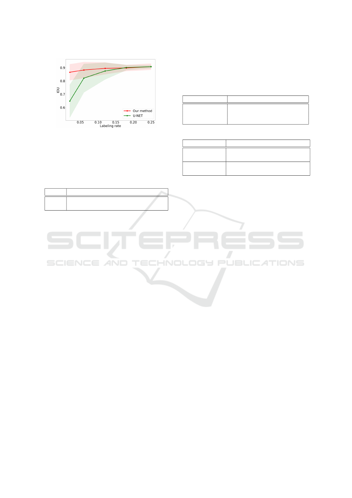
Figure 6: Mean IOU of our method (red) and U-Net (green)

when reconstructing the segmentation mask for the volume

with one partially labeled training slice for different labeling

rate. The green and red areas represent the standard devi-

ation of the results with U-Net and with our method (each

experiment is a 5-fold cross validation, repeated 5 times).

Table 2: Comparison of IOU between our method with both

loss combined and a U-Net architecture.

r 0.02 0.06 0.12 0.18 0.25

U-Net 0.648 0.821 0.875 0.902 0.908

Ours 0.866 0.883 0.895 0.898 0.908

4.3 Results

Study of Parameter r. We compare our method with

U-Net as a reference for different labeling rates to il-

lustrate the beneﬁt of learning an embedding space.

In addition to the 5-fold cross validation, each exper-

iment is repeated 5 times, resulting in a total of 25

realizations by experiment. The mean and standard

deviation are computed across these realizations. The

U-Net network is modiﬁed in order to make it com-

patible with partially labeled data like in C¸ ic¸ek et al.’s

work (C¸ ic¸ek et al., 2016) where a weighted cross-

entropy is used and unlabeled pixels’ weights are set

to 0. The results are shown in Figure 6 and in Table 2.

Our method performs signiﬁcantly better than U-Net

for small labeling rates, and has similar performance

for higher learning rate. The results are already perti-

nent, only using 2% of one labeled slice for training.

Comparison Study Between Supervised and Self-

Supervised Losses An ablation study was made to

study, for each labeling rate r the effect of activat-

ing either the supervised or the self-supervised loss

alone or the combination of both. As shown in Ta-

ble 3, when only the self-supervised loss is used,

the results are good even for a small labelling rate:

the latent space is well learned with only few anno-

tated pixels. As the labelling rate grows, only the

classiﬁcation layer beneﬁts from the supplementary

data. This results in little improvement as the la-

belling rate increases. The contrastive loss does not

perform well when only few data are provided, but

Table 3: Comparison of obtained mean IOU for indepen-

dent trainings by activating either the self-supervised, the

supervised or both losses (each experiment is a 5-fold cross

validation, repeated 5 times and the average is reported in

the table). Note that the classiﬁcation layer h is always

trained with supervision.

r 0.06 0.12 0.18 1.00

Self-Supervised 0.907 0.869 0.891 0.916

Supervised 0.773 0.875 0.861 0.926

Combined 0.883 0.895 0.898 0.927

Table 4: Results of our method for several volumes.

Zeolite 1 Zeolite 2 Alumina

U-Net r = 0.06 0.821 0.219 0.128

Ours r = 0.06 0.883 0.443 0.533

U-Net r = 0.25 0.908 0.392 0.196

Ours r = 0.25 0.908 0.595 0.729

as there are more labelled data, the supervised loss

performs better due to more diverse pairs of pixels.

When combining both supervised and self-supervised

loss, good results are obtained with a small labelling

rate, while performing better as the amount of labelled

data raises. Both supervised and self-supervised con-

trastive loss are required to obtain the best segmen-

tation. The whole reconstructed volume with both

losses combined can be seen in Figure 7.

Generalization to Other Volumes. Another vol-

ume of the same kind of zeolite (size 512×512×100)

and a volume of γ-alumina (Gay et al., 2016) (size

592×840×296) have also been segmented with our

approach. The results can be seen in Table 4. We

compared our method with both losses combined

against a U-Net like network. Our model performs

better than U-Net in most cases. Moreover, our

method reaches maximum values at a smaller label-

ing rate than U-Net, and performs better than U-Net

with very small values of r . The reconstruction of the

segmentation of the volume can be seen in Figure 7.

5 CONCLUSION

In this paper, we introduce a new semi-supervised

learning method for 3D image segmentation in elec-

tron tomography. Our model can achieve accurate

segmentation of electron tomography volumes with

only less than a slice for training data by using both

labeled and unlabeled data. Speciﬁcally, we com-

bine a contrastive path for labeled voxels and a self-

supervised path for unlabeled ones. This strategy

tends to maximize the possible use of all the informa-

tion available from the data. As the model can be built

on any 2D segmentation DL model, more modern ar-

Toward Few Pixel Annotations for 3D Segmentation of Material from Electron Tomography

129

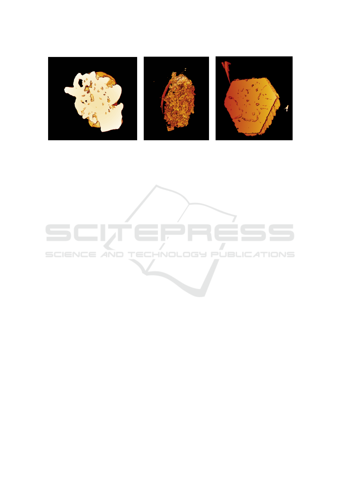
(1) (2) (3)

Figure 7: 3D reconstructions of the segmentation map of zeolites (1) (2) and γ-alumina (3). The volume (1) is cut to render

the inner structure of the volume. 6% of one slice has been taken to train the model used for each volume.

chitecture such as DeepLabV3+ (Chen et al., 2018b)

or UNet++ (Zhou et al., 2018) can be investigated for

future work. We have illustrated our strategy on elec-

tron tomography volume of material, but it is not lim-

ited to this type of data and acquisition, and could be

used in other ﬁelds as well, such as medical applica-

tions.

ACKNOWLEDGEMENTS

This work was supported by the LABEX MILYON

(ANR-10-LABX-0070) of Universit

e de Lyon, within

the program ”Investissements d’Avenir” (ANR-11-

IDEX- 0007) operated by the French National Re-

search Agency (ANR).

REFERENCES

Akers, S., Kautz, E., Trevino-Gavito, A., Olszta, M.,

Matthews, B. E., Wang, L., Du, Y., and Spurgeon,

S. R. (2021). Rapid and ﬂexible segmentation of elec-

tron microscopy data using few-shot machine learn-

ing. npj Computational Materials, 7(1):1–9.

Chaitanya, K., Erdil, E., Karani, N., and Konukoglu, E.

(2020). Contrastive learning of global and local fea-

tures for medical image segmentation with limited an-

notations. Advances in Neural Information Processing

Systems, 33:12546–12558.

Chen, L.-C., Papandreou, G., Kokkinos, I., Murphy, K.,

and Yuille, A. L. (2018a). Deeplab: Semantic im-

age segmentation with deep convolutional nets, atrous

convolution, and fully connected crfs. IEEE Trans-

actions on Pattern Analysis and Machine Intelligence,

40(4):834–848.

Chen, L.-C., Zhu, Y., Papandreou, G., Schroff, F., and

Adam, H. (2018b). Encoder-decoder with atrous sep-

arable convolution for semantic image segmentation.

Computer Vision – ECCV 2018, pages 833–851.

Chen, T., Kornblith, S., Norouzi, M., and Hinton, G. (2020).

A simple framework for contrastive learning of visual

representations. International conference on machine

learning, pages 1597–1607.

Chen, X. and He, K. (2021). Exploring simple siamese rep-

resentation learning. Proceedings of the IEEE/CVF

Conference on Computer Vision and Pattern Recogni-

tion (CVPR), pages 15750–15758.

C¸ ic¸ek,

O., Abdulkadir, A., Lienkamp, S. S., Brox, T.,

and Ronneberger, O. (2016). 3d u-net: Learning

dense volumetric segmentation from sparse annota-

tion. Medical Image Computing and Computer-

Assisted Intervention – MICCAI 2016, pages 424–

432.

Dosovitskiy, A., Springenberg, J. T., Riedmiller, M., and

Brox, T. (2014). Discriminative unsupervised fea-

ture learning with convolutional neural networks. Ad-

vances in neural information processing systems, 27.

Ersen, O., Hirlimann, C., Drillon, M., Werckmann, J., Ti-

hay, F., Pham-Huu, C., Cruciﬁx, C., and Schultz, P.

(2007). 3D-TEM characterization of nanometric ob-

jects. Solid State Sciences, 9(12):1088–1098.

Evin, B., Leroy,

E., Baaziz, W., Segard, M., Paul-Boncour,

V., Challet, S., Fabre, A., Thi

ebaut, S., Latroche,

M., and Ersen, O. (2021). 3D Analysis of Helium-

3 Nanobubbles in Palladium Aged under Tritium by

Electron Tomography. Journal of Physical Chemistry

C, 125(46):25404–25409.

Fernandez, J.-J. (2012). Computational methods for elec-

tron tomography. Micron, 43(10):1010–1030.

Flores, C., Zholobenko, V. L., Gu, B., Batalha, N., Valtchev,

V., Baaziz, W., Ersen, O., Marcilio, N. R., Ordomsky,

V., and Khodakov, A. Y. (2019). Versatile Roles of

Metal Species in Carbon Nanotube Templates for the

Synthesis of Metal–Zeolite Nanocomposite Catalysts.

ACS Applied Nano Materials, 2(7):4507–4517.

Frank, J. (2008). Electron tomography: methods for three-

dimensional visualization of structures in the cell.

Springer Science & Business Media.

VISAPP 2023 - 18th International Conference on Computer Vision Theory and Applications

130

Gay, A.-S., Humbert, S., Taleb, A.-L., Lefebvre, V.,

Dalverny, C., Desjouis, G., and Bizien, T. (2016).

Combined characterization of cobalt aggregates by

haadf-stem electron tomography and anomalous x-

ray scattering. European Microscopy Congress 2016:

Proceedings, pages 39–40.

Genc, A., Kovarik, L., and Fraser, H. L. (2022). A deep

learning approach for semantic segmentation of un-

balanced data in electron tomography of catalytic ma-

terials. arXiv preprint arXiv:2201.07342.

Grill, J.-B., Strub, F., Altch

e, F., Tallec, C., Richemond,

P. H., Buchatskaya, E., Doersch, C., Pires, B. A., Guo,

Z. D., Azar, M. G., Piot, B., Kavukcuoglu, K., Munos,

R., and Valko, M. (2020). Bootstrap Your Own Latent:

A new approach to self-supervised learning. Neural

Information Processing Systems.

Hadsell, R., Chopra, S., and LeCun, Y. (2006). Dimen-

sionality reduction by learning an invariant mapping.

2006 IEEE Conference on Computer Vision and Pat-

tern Recognition (CVPR’06), 2:1735–1742.

He, W., Ladinsky, M. S., Huey-Tubman, K. E., Jensen,

G. J., McIntosh, J. R., and Bj

orkman, P. J. (2008).

Fcrn-mediated antibody transport across epithelial

cells revealed by electron tomography. nature,

455(7212):542–546.

Kern, D., Klauck, U., Ropinski, T., and Mastmeyer, A.

(2021). 2D vs. 3D U-Net abdominal organ segmenta-

tion in CT data using organ bounds. Medical Imaging

2021: Imaging Informatics for Healthcare, Research,

and Applications, 11601:192 – 200.

Khadangi, A., Boudier, T., and Rajagopal, V. (2021). Em-

net: Deep learning for electron microscopy image seg-

mentation. 2020 25th International Conference on

Pattern Recognition (ICPR), pages 31–38.

Khosla, P., Teterwak, P., Wang, C., Sarna, A., Tian, Y.,

Isola, P., Maschinot, A., Liu, C., and Krishnan, D.

(2020). Supervised contrastive learning. Advances

in Neural Information Processing Systems, 33:18661–

18673.

Koch, G., Zemel, R., and Salakhutdinov, R. (2015).

Siamese neural networks for one-shot image recogni-

tion. ICML deep learning workshop, 2.

Li, X., Yu, L., Chen, H., Fu, C., and Heng, P. (2018). Semi-

supervised skin lesion segmentation via transforma-

tion consistent self-ensembling model. British Ma-

chine Vision Conference 2018, BMVC 2018, Newcas-

tle, UK, September 3-6, 2018, page 63.

Medeiros-Costa, I. C., Laroche, C., P

erez-Pellitero, J., and

Coasne, B. (2019). Characterization of hierarchi-

cal zeolites: Combining adsorption/intrusion, electron

microscopy, diffraction and spectroscopic techniques.

Microporous and Mesoporous Materials, 287:167–

176.

Milletari, F., Navab, N., and Ahmadi, S.-A. (2016). V-

net: Fully convolutional neural networks for volumet-

ric medical image segmentation. 2016 fourth interna-

tional conference on 3D vision (3DV), pages 565–571.

Ouali, Y., Hudelot, C., and Tami, M. (2020). Semi-

supervised semantic segmentation with cross-

consistency training. Proceedings of the IEEE/CVF

Conference on Computer Vision and Pattern Recogni-

tion, pages 12674–12684.

Pan, S. J. and Yang, Q. (2009). A survey on transfer learn-

ing. IEEE Transactions on knowledge and data engi-

neering, 22(10):1345–1359.

Peng, J., Estrada, G., Pedersoli, M., and Desrosiers, C.

(2020). Deep co-training for semi-supervised image

segmentation. Pattern Recognition, 107:107269.

Ronneberger, O., Fischer, P., and Brox, T. (2015). U-net:

Convolutional networks for biomedical image seg-

mentation. Medical Image Computing and Computer-

Assisted Intervention – MICCAI 2015, pages 234–

241.

Sun, K., Xiao, B., Liu, D., and Wang, J. (2019). Deep high-

resolution representation learning for human pose es-

timation. Proceedings of the IEEE/CVF Conference

on Computer Vision and Pattern Recognition, pages

5693–5703.

Volkmann, N. (2010). Methods for segmentation and in-

terpretation of electron tomographic reconstructions.

Methods in enzymology, 483:31–46.

Wurm, M., Stark, T., Zhu, X. X., Weigand, M., and

Taubenb

ock, H. (2019). Semantic segmentation of

slums in satellite images using transfer learning on

fully convolutional neural networks. ISPRS Journal

of Photogrammetry and Remote Sensing, 150:59–69.

Zhao, X., Vemulapalli, R., Mansﬁeld, P. A., Gong, B.,

Green, B., Shapira, L., and Wu, Y. (2021). Con-

trastive learning for label efﬁcient semantic segmen-

tation. Proceedings of the IEEE/CVF International

Conference on Computer Vision, pages 10623–10633.

Zhou, Z., Rahman Siddiquee, M. M., Tajbakhsh, N., and

Liang, J. (2018). Unet++: A nested u-net architecture

for medical image segmentation. In Deep learning in

medical image analysis and multimodal learning for

clinical decision support, pages 3–11. Springer.

Toward Few Pixel Annotations for 3D Segmentation of Material from Electron Tomography

131