Rotation Equivariance for Diamond Identification
Floris De Feyter
1 a
, Bram Claes
2
and Toon Goedem
´
e
1 b
1
EAVISE—PSI—ESAT, KU Leuven, Sint-Katelijne-Waver, Belgium
2
Antwerp Labs, Antwerp, Belgium
fl
Keywords:
Diamond Identification, Rotational Equivariance, Polar Warping.
Abstract:
To guarantee integrity when trading diamonds, a certified company can grade the diamonds and give them a
unique ID. While this is often done for high-valued diamonds, it is economically less interesting to do this
for lower-valued diamonds. While integrity could be checked manually as well, this involves a high labour
cost. Instead, we present a computer vision-based technique for diamond identification. We propose to apply
a polar transformation to the diamond image before passing the image to a CNN. This makes the network
equivariant to rotations of the diamond. With this set-up, our best model achieves an mAP of 100% under a
stringent evaluation regime. Moreover, we provide a custom implementation of the polar warp that is multiple
orders of magnitude faster than the frequently used implementation of OpenCV.
1 INTRODUCTION
To securely trade high-valued diamonds, the stones
are graded by a certified company like GIA and are
individually packed with a unique barcode. In some
cases, the unique ID is even engraved in the girdle
of the diamond. For smaller and lower-valued di-
amonds, this grading is economically less interest-
ing. Therefore, such diamonds are often not provided
with a unique ID. To make the trade of these smaller
diamonds—which make up the vast majority of di-
amonds sold—more secure, while keeping it cost-
effective, we propose to employ current computer vi-
sion techniques.
More specifically, we propose to train a Convolu-
tional Neural Network (CNN) to transform the im-
age of a diamond into a descriptive embedding—a
fingerprint—that can be used to compute a similarity
score for pairs of diamond images. Such an approach
has shown promising results for diamond identifica-
tion before (De Feyter et al., 2019). Instead of simply
training a CNN on our data, however, we propose to
modify the input images in such a way that the CNN
becomes rotation equivariant.
All diamonds in our dataset are photographed
from a top view, i.e., with their tables
1
parallel to the
camera sensor (see Fig. 3). Of course, apart from any
horizontal and vertical translation, a diamond is free
a
https://orcid.org/0000-0003-2690-0181
b
https://orcid.org/0000-0002-7477-8961
1
The flat part on top of the diamond.
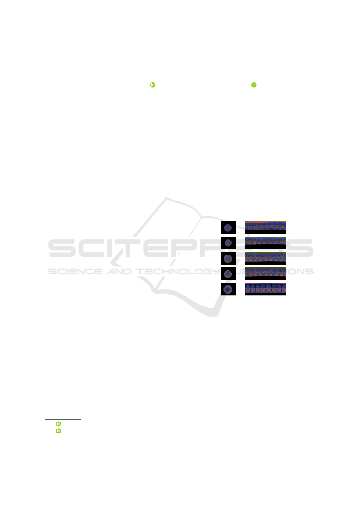
Original Polar warp
Figure 1: Polar warping applied to some random samples
from our dataset.
to have any rotation around the central axis perpen-
dicular to its table. A model that can match mul-
tiple images of the same diamond (each with a dif-
ferent orientation), therefore, must be insensitive to
these rotations. We propose to solve this by apply-
ing a polar warping operation to the diamond images
(see Fig. 1). Due to the nature of the polar warping,
a rotation of an object in an image results in a trans-
lation in the warped version of that image, as shown
in Fig 4. As the convolution operation is equivariant
to translations (Esteves et al., 2018), rotated versions
of the same diamond should yield similar outputs and
it should be easier to train a CNN for the task of dia-
mond identification. In Section 6.2, we show that the
addition of polar warping leads to models that achieve
100% mean Average Precision (mAP).
De Feyter, F., Claes, B. and Goedemé, T.
Rotation Equivariance for Diamond Identification.
DOI: 10.5220/0011658400003417
In Proceedings of the 18th International Joint Conference on Computer Vision, Imaging and Computer Graphics Theory and Applications (VISIGRAPP 2023) - Volume 5: VISAPP, pages
115-123
ISBN: 978-989-758-634-7; ISSN: 2184-4321
Copyright
c
 2023 by SCITEPRESS – Science and Technology Publications, Lda. Under CC license (CC BY-NC-ND 4.0)
115

While OpenCV (Bradski, 2000) contains an im-
plementation for such a polar transformation, it is not
suited for a deep learning pipeline. Therefore, in
Sec. 4.2, we develop our own implementation. Our
implementation supports GPU acceleration and can
perform the polar warp in batch. Moreover, the imple-
mentation allows for part of the transformation to be
precomputed. As we show in Sec. 6.3, this all leads to
a polar warp that—when executed on GPU—can run
750 times faster than OpenCV.
To summarize, the main contributions of this pa-
per are:
• The application of polar transformation to dia-
mond identification, with models reaching 100%
mAP for the identification of unseen diamonds;
• The implementation of a polar warp function that
is 750 times faster than the implementation of
OpenCV.
2 RELATED WORK
In this work, we employ rotation equivarience for im-
proving CNN-based diamond identification. The cur-
rent section discusses previous research on relevant
topics.
2.1 Gemstone Classification and
Identification
In (Chow and Reyes-Aldasoro, 2022), the authors
experimented with multiple feature extraction tech-
niques and machine learning algorithms, along with
ResNet-18 and ResNet-50 models (He et al., 2016) to
classify gemstone images of the Kaggle Gemstones
Images dataset (Chemkaeva, 2020). This dataset con-
tains more than 3200 images of 87 gemstone classes
(diamond, but also emerald, ruby, amethyst. . . ). In
their set-up, with an accuracy of 69.4%, the combi-
nation of a Random Forest algorithm and an RGB
eight-bin colour histogram and local binary features
turned out to be the most optimal. On this same
dataset, (Freire et al., 2022) finetuned an Inception-
v3 (Szegedy et al., 2015), achieving an accuracy of
72%. The models from these works, however, are
only capable of classifying in one of the 87 predefined
classes. We focus on a single type of gemstone, i.e.,
diamonds, and want the model to identify individual
stones. This implies that the model should generalize
to identifying diamonds it has not encountered during
training.
In the literature, we only found (De Feyter
et al., 2019) to employ computer vision tech-
niques for gemstone—or, more specifically dia-
mond—identification. Here, the authors finetune a
Darknet-19 backbone (Redmon and Farhadi, 2016)
that was pretrained on ImageNet (Deng et al., 2009).
They report a top-1 accuracy of 99.7%. Their vali-
dation set, however, contains different images from
the same diamonds as were used during training. We
believe that the only way to truly evaluate the gen-
eralization of an identification system is by validat-
ing on different identities than those that were used
during training. Similar to (De Feyter et al., 2019),
we finetune a CNN that was pertrained on ImageNet.
We use a different model, however, that outputs more
compact embeddings with 512 floating point numbers
instead of 1024. Additionally, we demonstrate that a
polar warping operation notably improves the CNN
baseline.
2.2 Rotation Equivariance for CNNs
An important aspect of the solution we propose to di-
amond identification, is to make the model equivari-
ant to rotations of the diamond. Making a CNN ro-
tation equivariant has been studied before. In (Hen-
riques and Vedaldi, 2017), the authors present a gen-
eral approach to make CNNs equivariant to a set of
two-parameter transformations, among which rota-
tion (and scale). The equivarience is attained by warp-
ing the input image, based on a flow grid that is de-
fined by the nature of the two-parameter transforma-
tion. The Polar Transform Network (PTN) introduced
by (Esteves et al., 2018) focuses on rotation equiv-
ariance only. Their network predicts a polar origin
and uses this to warp the input image around that ori-
gin. The warped image is passed to a conventional
CNN classifier. In our application, however, it is rela-
tively easy to find a good polar origin and as such, we
can avoid the extra complexity of an origin predictor
network. Similar to (Kim et al., 2020), instead, we di-
rectly apply a polar transform to the input image with-
out passing the image through an origin predictor first.
The polar origin used by (Kim et al., 2020), however,
is defined as the image center. To limit the changes
in the appearance of a diamond in the warped view,
we choose to use the diamond centroid as polar origin
instead. In their implementation, (Kim et al., 2020)
make use of the OpenCV function warpPolar(). We
have implemented our own polar transformation func-
tion that can process image batches on GPU and as
such is more than 750 times faster than the OpenCV
implementation (see Sec. 6.3).
VISAPP 2023 - 18th International Conference on Computer Vision Theory and Applications
116

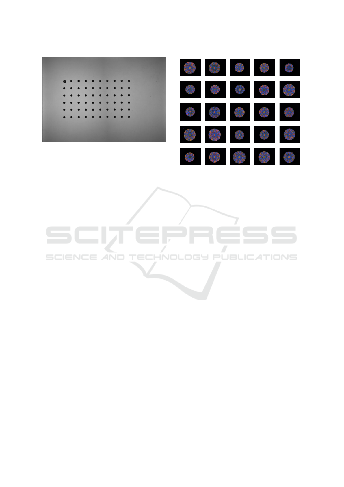
Figure 2: Example of how we arranged a batch of diamonds
during data collection.
3 DATASET
We developed a large dataset suitable for training
a CNN for diamond identification. Our dataset is
an order of magnitude larger than the one used by
(De Feyter et al., 2019). Apart from better training,
this allows for a more stringent and more accurate
evaluation. Due to the high value of diamonds, er-
roneously matching diamonds might lead to signifi-
cant losses. Therefore, an accurate evaluation of our
model is crucial in this application.
3.1 Data Collection
In order to collect a large dataset, we have built a set-
up that can automatically process diamonds in batch.
The set-up consists of a robot arm, a rotating glass
disk, a light source and a camera mounted on a fixed
height above the glass plate. The whole set-up is en-
closed such that no light can enter from outside. A
batch of diamonds is manually prepared in an array
as shown in Fig. 2. A camera mounted on the robot
arm scans this array and detects where the diamonds
are positioned. One by one, the robot arm grabs a first
set of diamonds and lays them on the rotating disk.
The disk stops rotating once a diamond passes under
the fixed camera after which the light source projects
a colour pattern through the diamond and a picture
is taken. Inspired by (De Feyter et al., 2019), we
have designed this colour pattern to produce specif-
ically colour-coded diamond images, as can be seen
in Fig. 3. Once a diamond has been photographed,
the robot arm picks it up from the glass plate and puts
it back in the array. When all diamonds in the array
are photographed, the whole procedure is repeated N
times to have N photographs per diamond.
Figure 3: Some random samples from our dataset.
3.2 Dataset Properties
Via the procedure described in Sec. 3.1, we were
able to compose a dataset with 96385 RGB images
of 1021 diamonds. The images have a resolution of
2448×2048 pixels. We split up this dataset in a train-
ing dataset with 77 060 images of 816 diamonds and
a validation dataset with 19 325 images of 205 dia-
monds. Note that not only the set of training images
and the set of validation images, but also the sets of di-
amond identities are disjoint. Fig 3 shows some sam-
ples from our dataset. For our experiments (Sec. 6),
the validation dataset is split up further into a query
and a gallery set. The gallery set contains 10 images
of each diamond, the query set contains the rest of the
validation images.
4 POLAR WARPING
In our application, the orientation of the diamond in
an image is meaningless. Hence, our model should be
robust against diamond rotations. By applying a po-
lar warp to the input image, rotations of the diamond
can be transformed to translations, to which a CNN
is equivariant (Esteves et al., 2018; Kim et al., 2020).
Therfore, with polar warping, the CNN can be made
equivariant to the diamond rotations by design.
For their CyCNN, (Kim et al., 2020) make
use of the polar warp function implemented in
OpenCV (Bradski, 2000), i.e., warpPolar(). This
implementation, however, is not suited for a typical
deep learning set-up. It cannot perform the polar warp
on GPU, let alone apply the transformation to a batch
of images. So, to process a batch of images that is
Rotation Equivariance for Diamond Identification
117

Cartesian Polar
Figure 4: Toy example of applying a polar warp to rotated
version of the same object. The center of the emoji is chosen
as polar origin and the polar radius is chosen equal to the
radius of the emoji’s head. As the emoji rotates, the polar
warp shifts horizontally.
loaded into GPU memory, we would need to move the
batch to CPU, pass each image individually through
warpPolar(), put the results into a batch and move
that batch back to GPU memory. This clearly is a
wasteful round trip. One way to avoid this would be
to apply the polar warp to the entire dataset offline
and load the warped image directly into GPU mem-
ory. This is undesirable, however, as it makes some
data augmentations difficult to perform during train-
ing, e.g., random cropping, random rotation or ran-
domly offsetting the polar origin. Also, this would
require a lot more storage as each image will have a
regular and a warped version.
4.1 Formal Definition of Polar Warping
Let ⃗p be the position of a point in an image. The polar
coordinates (φ, ρ) of this point with respect to some
point at ⃗c (which we call the polar origin), then, are
defined as:

φ = ∠ (⃗p −⃗c)
ρ = ∥⃗p −⃗c∥,
(1)
with φ ∈ [0,2π[ and ρ ∈ R
+
. This definition can
be reformulated to express the Cartesian coordinates
of points in the input image as a function of their polar
coordinates (φ,ρ). Let (x,y) and (c
x
,c
y
) be the Carte-
sian coordinates of ⃗p and ⃗c, respectively. Then, from
Eqn. 1 it follows that,







cosφ =
x − c
x
ρ
⇐⇒ x = c
x
+ ρ · cosφ
sinφ =
y − c
y
ρ
⇐⇒ y = c
y
+ ρ · sinφ.
(2)
It is customary to limit ρ ∈ [0,R], with polar ra-
dius R and R ∈ R
+
, such that the mapped points all lie
in a circle with center at⃗c and radius R and the output
of the transformation will have a rectangular shape.
4.2 Implementation
A standard way to implement geometric transforma-
tions in software is by defining a flow field grid G .
Let I be the input image of shape (W, H,C) and I
′
be
the warped output image of shape (W
′
,H
′
,C). Then,
the flow field grid has shape (W
′
,H
′
,2), i.e., it has
the same width and height as I
′
, but instead of color
channels, G consists of an x and a y channel. The
(x,y) value stored at a certain location (u,v) in G de-
scribes the coordinates of the point in I that should
come at location (u,v) in I
′
. Note that the coordinates
stored in G is typically non-integer, and an interpola-
tion of multiple pixel values is used to compute an
output pixel value.
To compose G for a polar mapping, we first create
two arrays of evenly spaced numbers. For φ, this array
contains numbers in the interval [0,2π[ and has length
W
′
, i.e., the output width. For ρ, the numbers are
in [0,R] and the array’s length is equal to the output
height H
′
. Now let ∆φ and ∆ρ be the step sizes used
in the arrays for φ and ρ, respectively. Then, from
Eqn. 2, we find that the value at location (u, v) in G,
with u ∈ {0,1, .. .,W
′
− 1} and v ∈ {0,1, .. ., H
′
− 1},
should be equal to

G
x
(u,v) = c
x
+ v∆ρ · cos(u∆φ)
G
y
(u,v) = c
x
+ v∆ρ · sin(u∆φ),
(3)
where G
x
and G
y
are the x and y channel of
G, respectively. By passing G to a function like
grid_sample() in PyTorch (Paszke et al., 2019),
along with the input image I , we apply the polar map-
ping to I and obtain I
′
.
4.3 Improved Implementation with
Fixed Polar Radius
From Eqn. 3, we can see that the flow field grid G
used to perform the polar warp consists of two terms,
one depends on polar origin ⃗c and one depends on
the array of values used for ρ and φ. Hence, when
applying a polar warp multiple times with the same
values for ρ, the second term can be precomputed (the
values used for φ are assumed to be constant). We
define a base grid
ˆ
G such that the value at location
(u,v) is given by
(
ˆ
G
x
(u,v) = v∆ρ · cos (u∆φ)
ˆ
G
y
(u,v) = v∆ρ · sin (u∆φ).
(4)
VISAPP 2023 - 18th International Conference on Computer Vision Theory and Applications
118

Then, any G can be easily computed from
ˆ
G by
simply adding the coordinates of the polar origin,
(
G(u,v) = c
x
+
ˆ
G
x
(u,v)
G(u,v) = c
y
+
ˆ
G
y
(u,v).
(5)
Algorithm 1 shows pseudocode for the precompu-
tation of G, while Algorithm 2 shows how the polar
mapping is performed from a precomputed flow field
grid.
Algorithm 1: Precomputing the Base Flow Field Grid.
procedure BASE GRID(width, height, R)
∆φ ← 2π/width ▷ Define step size
∆ρ ← R/height
φ ← [0 : ∆φ : 2π[ ▷ Define φ, ρ as row vectors
ρ ← [0 : ∆ρ : R]
ˆ
G
x
← ρ
T
cosφ ▷ Compute both channels of
ˆ
G
ˆ
G
y
← ρ
T
sinφ
return
ˆ
G
Algorithm 2: Polar Mapping with Precomputed Flow Field
Grid.
procedure POLAR MAP(I ,
ˆ
G,c
x
,c
y
)
G
x
← c
x
+
ˆ
G
x
▷ Compute both channels of G
G
y
← c
y
+
ˆ
G
y
I
p
= grid_sample(I ,G )
return I
p
5 POLAR WARPING FOR
DIAMOND IDENTIFICATION
As discussed in Section 4, applying a polar warping
operation to an image requires two parameters: a po-
lar origin ⃗c and a polar radius R. In Sec. 5.1, we mo-
tivate why one would choose the diamond centroid to
be the polar origin and how we can reliably find this
centroid in each image. In Sec. 5.2, we discuss how
we can determine a (fixed) polar radius.
5.1 Diamond Centroid as Polar Origin
The closer a region is to the polar origin in the input
image I , the more space it will occupy in the warped
image I
′
. The centroid of the diamond is the point
where the sum of distances to all points on the dia-
mond is minimized, so, the centroid seems like a good
choice for the polar origin, as this will maximize the
amount of pixels in I
′
that contain information of the
diamond. Moreover, the centroid of the diamond can
easily and reliably be retrieved in the images of our
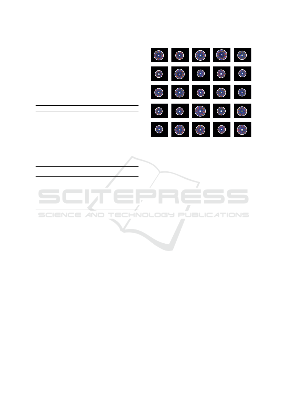
Figure 5: The detected center and estimated radius for 25
random samples from our dataset.
dataset, which is important to have transformed ver-
sions of the same diamond only differ by a horizontal
shift.
As can be seen in Fig. 3, the diamonds are clearly
visible against the black background. This sug-
gests that classic computer vision techniques should
suffice to detect the centroid. Indeed, a sim-
ple binary threshold is enough to segment the dia-
mond from the background. By applying OpenCV’s
findContours() (Bradski, 2000) on the binarized
image and selecting the contour with the largest area,
we can draw a boundary around the diamond. Next,
via OpenCV’s moments() function, we can retrieve
the coordinates of the diamond’s centroid. Fig. 5
shows some examples of the diamonds and centroids
that were detected in this way. We store each dia-
mond’s centroid and radius information in a separate
file that accompanies the respective image. In each
image, the detection algorithm found exactly one cen-
troid. A visual check of hundreds of random samples
confirmed that the algorithm was able to correctly de-
tect the diamond boundaries and centroids.
5.2 Fixed Polar Radius
A desirable by-product of our centroid detection
method is that the radii of the diamonds are also mea-
sured. Figure 6 shows the distribution of all radii. For
the polar radius R, one option would be to adapt the
radius to the size of the diamond so that each dia-
mond would approximately take up the same space
in the warped image. This would make the model less
sensitive to scale changes in diamond images. How-
ever, a different scale could be an easy way for our
model to know that two diamonds are different. Our
Rotation Equivariance for Diamond Identification
119

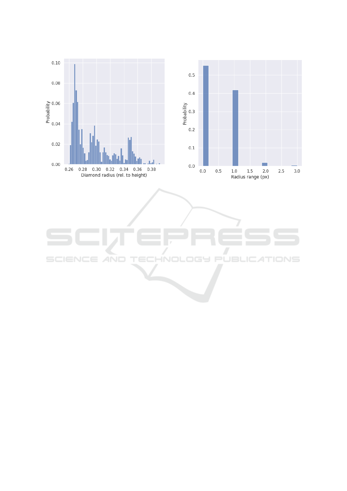
Figure 6: The distribution of the estimated radii of the dia-
monds in our dataset. The radii are expressed relative to the
image height.
system always photographs the diamonds from the
same distance, so a diamond should have a consistent
scale across all images. Indeed, when we compute
the difference between the largest and smallest radius
of each diamond (see Fig. 7), we find that for 97.4%
of the diamonds, there is no more than 1 pixel differ-
ence. Furthermore, there are no diamonds for which
the difference is larger than 3 pixels.
From Fig. 6, we know that there are no dia-
monds larger than about 40% of the image height.
As we resize the images to a height of 256 pixels,
this corresponds to about 100 pixels. Adding in some
head space, we fix the polar radius R at 112 pixels.
Note that, with this fixed value for R, we open the
door to the implementation improvement described in
Sec. 4.3.
6 EXPERIMENTS AND RESULTS
This section presents our experimental set-up and re-
sults. In Sec. 6.1, we provide the implementation de-
tails of the models and describe how we train them for
diamond identification. We apply multiple ablations
to our baseline model, among which polar warping of
the input, and report the results in Sec. 6.2. Finally, in
Sec. 6.3, we compare our polar warp implementation
with OpenCV’s warpPolar().
Figure 7: The distribution of the range of the estimated radii
across the images of each individual diamond in our dataset.
6.1 Model Implementation Details
For all our experiments, we employ a ResNet-18
model (He et al., 2016) that was pretrained on Ima-
geNet (Deng et al., 2009). We allow all weights to
train (no frozen layers). We use Stochastic Gradient
Descent (SGD) to optimize the weights with a learn-
ing rate of 0.1, a momentum of 0.95 and no weight
decay. We apply a linear learning rate warm-up for
the first 400 iterations (Goyal et al., 2017) and half the
learning rate after 6 and 9 epochs. We limit the num-
ber of epochs to 10, as none of our models showed
any further improvement after that. All models are
trained on a single NVIDIA Tesla V100 GPU.
The model outputs an embedding of length 512.
During model training, however, we append an ex-
tra trainable fully-connected layer that transforms this
embedding to a vector with the same length as the
number of training classes. From this, we can com-
pute the softmax cross-entropy loss. As such, the
model is de facto trained as a classifier and the em-
bedding is trained implicitly. Note that, during vali-
dation, this fully-connected layer is not used.
We split up the dataset into a training, a valida-
tion gallery and a validation query set as described
in Sec. 3.2. We use a batch size of 60 images for
training and validation. The images are resized to a
height of 256 pixels. After resizing, a random square
region of 224 pixels wide is cropped out of each im-
age. The validation data is center cropped to the same
size. Then, the image is normalized with either Im-
ageNet (Deng et al., 2009) statistics or the mean and
VISAPP 2023 - 18th International Conference on Computer Vision Theory and Applications
120

standard deviation of the pixel values in the training
set. In some experiments, we also apply a random ro-
tation to the training images. This is done before the
random crop. Note that each image is accompanied
by a file that contains the coordinates of the diamond
centroid (see Sec. 5.2). These coordinates are trans-
formed along so that the polar transformation can be
correctly applied to the input batch. Polar warping
is performed after the data transformation pipeline.
Note that the coordinates of the centroid are trans-
formed along with the image so that the position of
the centroid does not change relative to the diamond.
6.2 Ablation Study
We explore the effect of adding the polar warping de-
scribed in Sec. 4, along with other hyperparameters.
Table 1 summarizes this ablation experiment. We re-
port the mAP after one epoch of training and after ten
epochs of training, averaged over 5 runs (mean ± std.
dev.). To compute the mAP, we first pass both the
query images and the gallery images (see Sec. 3.2)
through the model, obtaining an embedding for each
image. Then, we compute a similarity matrix between
the query embeddings and the gallery embeddings
from their cosine similarities. For every query, we
sort the similarities from most to least similar to the
query. From these sorted similarity sequences, along
with the ground truth query and gallery labels, we can
compute an AP for each query. The mAP is then ob-
tained by averaging all APs.
From Table 1, we can see that when the base-
line is trained with random resized cropping (Base-
line+RRC), the model performs significantly worse
than when we apply random cropping without ran-
dom resizing (Baseline). Note that random resized
cropping involves that the input images are first re-
sized to a random size, after which a random region
of a fixed size is cropped out. This data augmentation
technique is typically used to make a model invariant
to scale changes. However, due to our camera set-up,
the same diamond will always have the same scale in
the image and the model can safely use the scale of
a diamond as a descriptive feature. This is confirmed
by the drop of more than 10 percent points when we
add random resized cropping to the baseline.
A slight increase in mAP after 1 epoch of train-
ing is found when we replace ImageNet normaliza-
tion with the mean and standard deviation of the dia-
mond dataset itself (Baseline+Norm). The images in
our dataset contain a lot more dark areas than typi-
cal ImageNet (Deng et al., 2009) images. Therefore,
the mean red, green and blue pixel values are much
smaller than in ImageNet. After 10 epochs, however,
as the BatchNorm (Ioffe and Szegedy, 2015) layers in
the model adapted to the data distribution, the mAP
difference with the baseline becomes negligible.
The largest increase with respect to the baseline
is seen when the input is transformed with the polar
mapping presented in Sec. 4 (Baseline+Norm+Polar
and Baseline+Norm+Rot+Polar), with an addi-
tional increase when we add random rotations.
Note that these random rotations result in random
horizontal shifts of the diamond in the warped
image. During training, there were two individ-
ual runs—one Baseline+Norm+Polar model, one
Baseline+Norm+Rot+Polar—that achieved 100%
mAP. These models are able to find, for each of
17 480 query images of unseen diamonds, the 10 out
of 2050 gallery images of the same diamond. None
of the other methods had a run that performed so well
anytime during training.
This result greatly surpasses the result of
(De Feyter et al., 2019), who needed a kNN with k = 5
to finally achieve 100% mAP on their tiny dataset of
64 diamond classes.
As shown in Table 2, it takes about 1/3 longer
to train 10 epochs when polar transformation is per-
formed before passing the input to the model. How-
ever, from Table 1 we know that, after only a single
epoch, models with polar transformation already per-
form on par with non-polar methods trained for 10
epochs. So, in an mAP per time sense, the polar meth-
ods clearly outperform the non-polar methods.
6.3 Polar Warp Comparison
We measure the duration of our polar warp im-
plementation (see Sec. 4.2) under different settings
and compare it to the warpPolar() function of
OpenCV (Bradski, 2000). We select 16 random im-
ages from our dataset (size 2448 × 2048) and apply
a polar transformation using the detected centroid of
the diamond (see Sec. 5.2) as polar origin and a fixed
radius of 1024. As can be seen from Table 3, our Py-
Torch implementation runs about 1.2 times faster than
OpenCV on CPU (Intel Xeon E5-2630 v2) and more
than 200 times faster on GPU (NVIDIA GeForce
GTX 1180). When precomputing a base flow grid,
as presented in Sec. 4.2, our method runs even 750
times faster than OpenCV. The polar warps created
by OpenCV and by our own PolarTorch are visually
identical, as demonstrated in Fig. 8. When subtract-
ing the pixel values of outputs from both implemen-
tations, we found some differences, though, but we
consider these negligible.
Rotation Equivariance for Diamond Identification
121

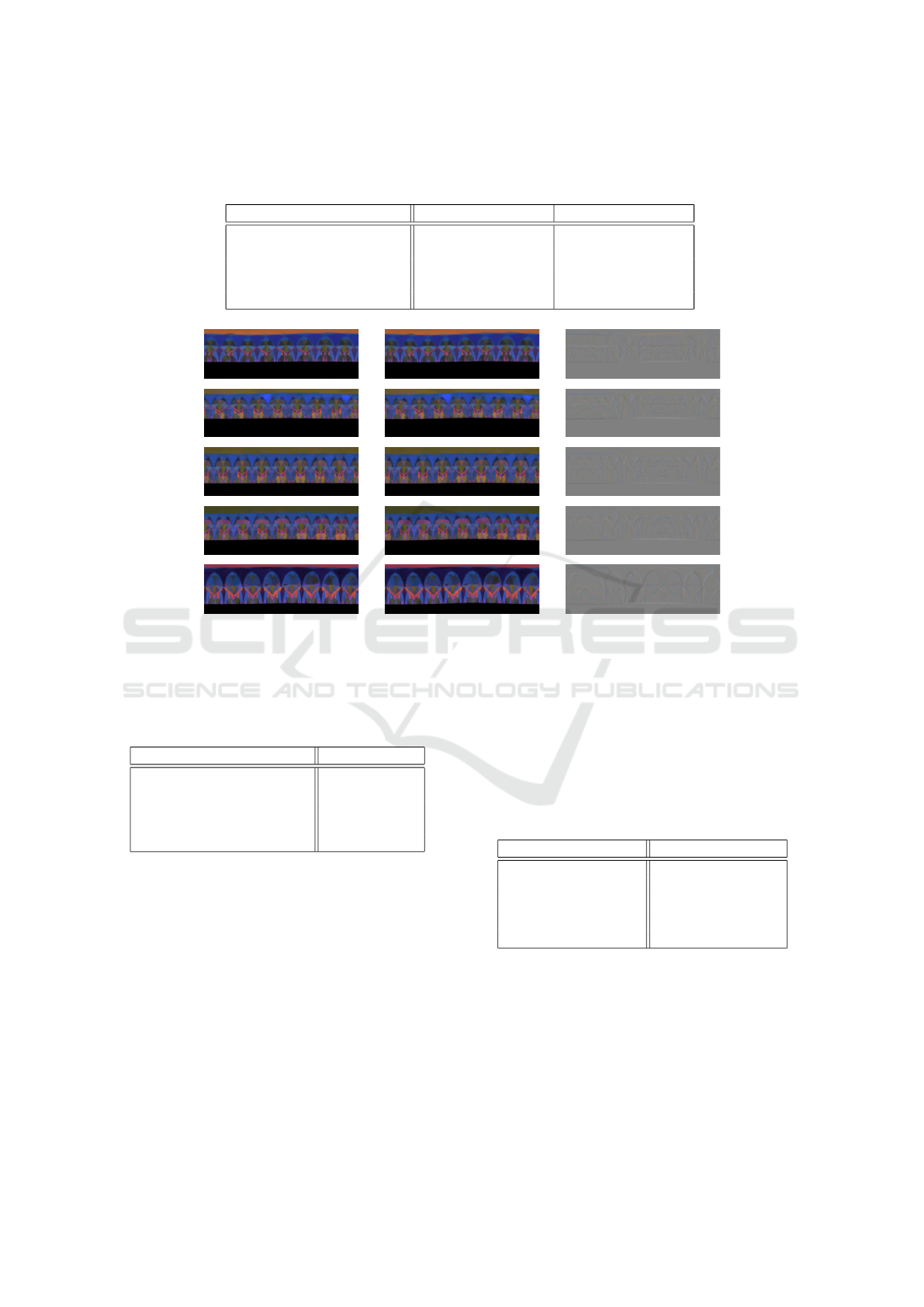
Table 1: Results of the ablation study. The results are reported as mAP on the validation set after 1 and 10 epochs. Each
configuration is trained 5 times; we report the mean and std. dev. RRC: Random Resized Crop; Norm: Normalized with
statistics of our own dataset; Rot: Random Rotation augmentation; Polar: With polar warping applied.
Method mAP, ep 1 (%) mAP, ep 10 (%)
Baseline 99.31597 ± 0.18825 99.96971 ± 0.01056
Baseline+RRC 97.59266 ± 0.76504 99.63744 ± 0.12250
Baseline+Norm 99.69073 ± 0.10654 99.96785 ± 0.02039
Baseline+Norm+Polar 99.93370 ± 0.02317 99.98011 ± 0.02720
Baseline+Norm+Rot+Polar 99.93151 ± 0.05273 99.98864 ± 0.00994
cv.warpPolar() Our polar warp Difference
Figure 8: Applying OpenCV’s and our implementation of a polar warp to 5 samples from our dataset. The right-hand column
shows the difference between both outputs, with pixel values shifted and scaled to fall in range [0, 255], i.e., gray means 0
difference.
Table 2: Training duration (10 epochs) of the ablation con-
figurations.
Method Time (10 eps.)
Baseline 21’10” ± 21”
Baseline+RRC 21’40” ± 32”
Baseline+Norm 21’34” ± 29”
Baseline+Norm+Polar 28’36” ± 33”
Baseline+Norm+Rot+Polar 28’27” ± 34”
7 CONCLUSION
We have shown that a CNN is well suited for diamond
identification. When applying a polar transformation
to the input image, with the diamond’s centroid as po-
lar origin and a fixed predefined radius, the CNN can
be trained to perform better in less epochs. Our cus-
tom polar warp implementation significantly reduces
the computation time when compared to OpenCV’s
implementation, up to a factor 750. Our best models
achieved an mAP of 100%, i.e., they were able to find,
for each of 17 480 images of unseen diamonds the 10
out of 2050 gallery images of the same diamond.
Table 3: Duration (mean ± std. dev. for 10 runs) for per-
forming a polar warp of 16 images of size 2448× 2048 with
different methods. The CPU methods are executed on an
Intel Xeon E5-2630 v2 (2.60 GHz), the GPU methods on
an NVIDIA GeForce GTX 1180. “
ˆ
G” indicates that the
method uses a precomputed flow field (see Sec. 4.2). The
PolarTorch implementation on GPU with a precomputed
flow field is more than 750 times faster than OpenCV.
Method Time for 16 images
OpenCV (CPU) 825.3 ms ± 7.9 ms
PolarTorch (CPU) 668.4 ms ± 8.5 ms
PolarTorch (CPU,
ˆ
G) 642.1 ms ± 30.8 ms
PolarTorch (GPU) 3.7 ms ± 0.2 ms
PolarTorch (GPU,
ˆ
G) 1.1 ms ± 1.3 ms
REFERENCES
Bradski, G. (2000). The OpenCV library. Dr. Dobb’s Jour-
nal of Software Tools.
Chemkaeva, D. (2020). Gemstones Images.
https://www.kaggle.com/datasets/lsind18/gemstones-
images.
VISAPP 2023 - 18th International Conference on Computer Vision Theory and Applications
122

Chow, B. H. Y. and Reyes-Aldasoro, C. C. (2022). Au-
tomatic Gemstone Classification Using Computer Vi-
sion. Minerals, 12(1):60.
De Feyter, F., Hulens, D., Claes, B., and Goedeme, T.
(2019). Deep Diamond Re-ID. In 2019 18th IEEE
International Conference On Machine Learning And
Applications (ICMLA), pages 2020–2025.
Deng, J., Dong, W., Socher, R., Li, L., Kai Li, and Li Fei-
Fei (2009). ImageNet: A large-scale hierarchical im-
age database. In 2009 IEEE Conference on Computer
Vision and Pattern Recognition, pages 248–255.
Esteves, C., Allen-Blanchette, C., Zhou, X., and Dani-
ilidis, K. (2018). Polar Transformer Networks.
arXiv:1709.01889 [cs].
Freire, W. M., Amaral, A. M. M. M., and Costa, Y. M. G.
(2022). Gemstone classification using ConvNet with
transfer learning and fine-tuning. In 2022 29th Inter-
national Conference on Systems, Signals and Image
Processing (IWSSIP), volume CFP2255E-ART, pages
1–4.
Goyal, P., Doll
´
ar, P., Girshick, R., Noordhuis, P.,
Wesolowski, L., Kyrola, A., Tulloch, A., Jia, Y., and
He, K. (2017). Accurate, Large Minibatch SGD:
Training ImageNet in 1 Hour.
He, K., Zhang, X., Ren, S., and Sun, J. (2016). Deep Resid-
ual Learning for Image Recognition. In The IEEE
Conference on Computer Vision and Pattern Recog-
nition (CVPR), pages 770–778, Las Vegas, NV, USA.
IEEE.
Henriques, J. F. and Vedaldi, A. (2017). Warped Convolu-
tions: Efficient Invariance to Spatial Transformations.
In Proceedings of the 34th International Conference
on Machine Learning, pages 1461–1469. PMLR.
Ioffe, S. and Szegedy, C. (2015). Batch Normalization: Ac-
celerating Deep Network Training by Reducing Inter-
nal Covariate Shift. arXiv:1502.03167 [cs].
Kim, J., Jung, W., Kim, H., and Lee, J. (2020). CyCNN:
A Rotation Invariant CNN using Polar Mapping and
Cylindrical Convolution Layers. arXiv:2007.10588
[cs, eess].
Paszke, A., Gross, S., Massa, F., Lerer, A., Bradbury, J.,
Chanan, G., Killeen, T., Lin, Z., Gimelshein, N.,
Antiga, L., Desmaison, A., K
¨
opf, A., Yang, E., De-
Vito, Z., Raison, M., Tejani, A., Chilamkurthy, S.,
Steiner, B., Fang, L., Bai, J., and Chintala, S. (2019).
PyTorch: An Imperative Style, High-Performance
Deep Learning Library.
Redmon, J. and Farhadi, A. (2016). YOLO9000: Better,
Faster, Stronger. arXiv:1612.08242 [cs].
Szegedy, C., Vanhoucke, V., Ioffe, S., Shlens, J., and Wojna,
Z. (2015). Rethinking the Inception Architecture for
Computer Vision.
Rotation Equivariance for Diamond Identification
123