Robust RGB-D-IMU Calibration Method Applied to GPS-Aided Pose

Estimation

Abanob Soliman

∗ a

, Fabien Bonardi

§ b

, D

esir

e Sidib

§ c

and Samia Bouchafa

§ d

Universit

e Paris-Saclay, Univ. Evry, IBISC Laboratory, 34 Rue du Pelvoux, Evry, 91020, Essonne, France

∗

ﬁ ﬁ

Keywords:

RGB-D Cameras, Calibration, RGB-D-IMU, Bundle-Adjustment, Optimization, GPS-Aided Localization.

Abstract:

The challenging problem of multi-modal sensor fusion for 3D pose estimation in robotics, known as odometry,

relies on the precise calibration of all sensor modalities within the system. Optimal values for time-invariant

intrinsic and extrinsic parameters are estimated using various methodologies, from deterministic ﬁlters to non-

deterministic optimization models. We propose a novel optimization-based method for intrinsic and extrinsic

calibration of an RGB-D-IMU visual-inertial setup with a GPS-aided optimizer bootstrapping algorithm. Our

front-end pipeline provides reliable initial estimates for the RGB camera intrinsics and trajectory based on

an optical ﬂow Visual Odometry (VO) method. Besides calibrating all time-invariant properties, our back-

end optimizes the spatio-temporal parameters such as the target’s pose, 3D point cloud, and IMU biases.

Experimental results on real-world and realistically high-quality simulated sequences validate the proposed

ﬁrst complete RGB-D-IMU setup calibration algorithm. Ablation studies on ground and aerial vehicles are

conducted to estimate each sensor’s contribution in the multi-modal (RGB-D-IMU-GPS) setup on the vehicle’s

pose estimation accuracy. GitHub repository: https://github.com/AbanobSoliman/HCALIB.

1 INTRODUCTION

A reliable autonomous vehicle odometry solution re-

lies on the continuous availability of the scene and

vehicle information, such as scene structure and the

vehicle’s physical properties (position, velocity, or ac-

celeration). These properties are measured by exte-

roceptive (Cameras/LiDAR/Radar/GPS) and propri-

oceptive (IMU/Wheel odometry) sensor modalities.

Hence, multi-modal odometry algorithms have at-

tracted the attention of many researchers in the last

few years (Hug et al., 2022; Chghaf et al., 2022;

Chang et al., 2022; Jung et al., 2022), especially in

challenging low structured environments.

Solutions incorporating a multi-camera system

with no IMUs can be much easier to bootstrap using

the 5-point (Nist

er, 2004) or the 8-point (Heyden and

Pollefeys, 2005) SfM algorithms with a robust out-

lier ﬁltration method (Antonante et al., 2021; Barath

et al., 2020) without the need to estimate a global met-

ric scale for the trajectory.

Adding an IMU (or multiple IMUs as in (Rehder

https://orcid.org/0000-0003-4956-8580

https://orcid.org/0000-0002-3555-7306

https://orcid.org/0000-0002-5843-7139

https://orcid.org/0000-0002-2860-8128

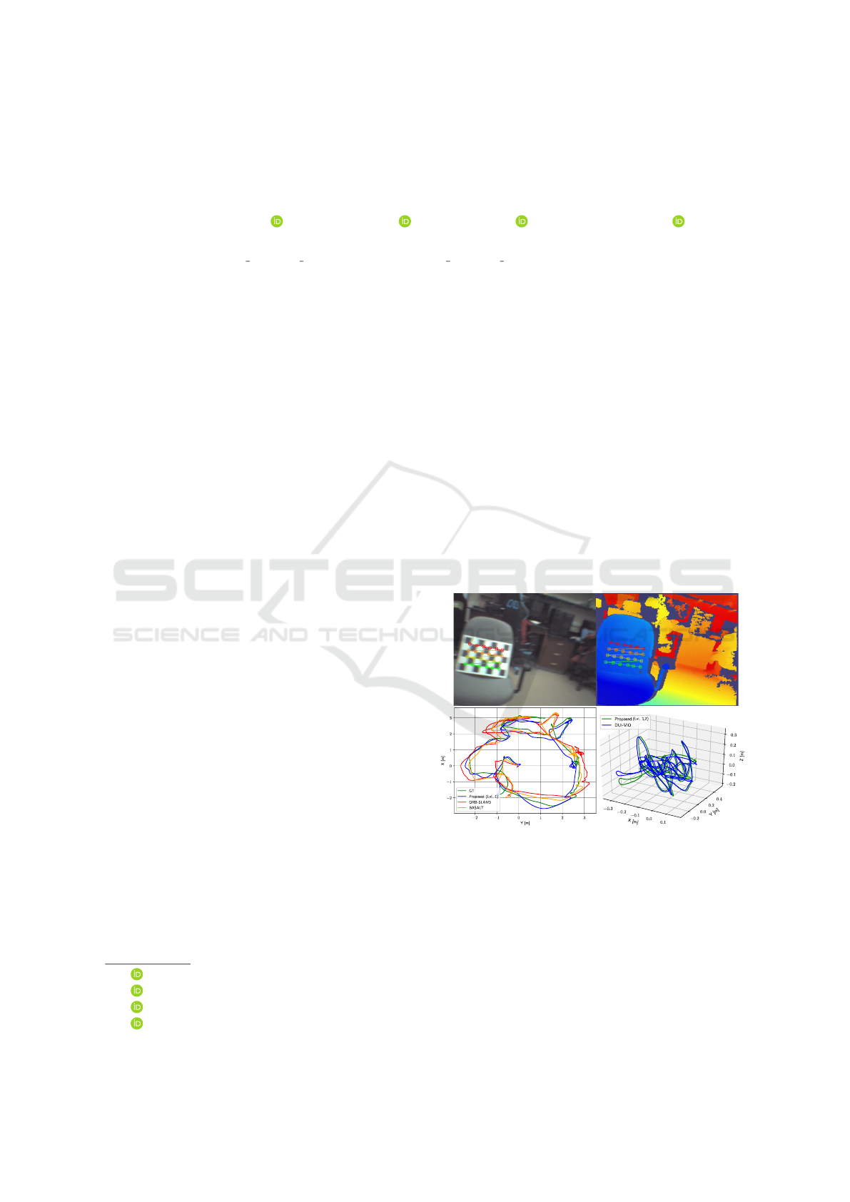
Figure 1: Our RGB-D-IMU setup calibration and pose es-

timation pipeline applied to the VCU-RVI hand-eye cali-

bration sequence (top/bottom-right) and the EuRoC V2-01

sequence (bottom-left).

et al., 2016)) to a multi-camera calibration framework

increases the complexity in the alignment process of

the target’s initial arbitrarily scaled poses with the ini-

tial real-world metric scaled ones (Qin et al., 2018).

In the recent work of (Das et al., 2021), they studied

a graph-based optimization approach that fuses GPS

and IMU readings with stereo-RGB cameras. They

show a superior estimation accuracy, especially in an

Soliman, A., Bonardi, F., Sidibé, D. and Bouchafa, S.

Robust RGB-D-IMU Calibration Method Applied to GPS-Aided Pose Estimation.

DOI: 10.5220/0011656800003417

In Proceedings of the 18th International Joint Conference on Computer Vision, Imaging and Computer Graphics Theory and Applications (VISIGRAPP 2023) - Volume 4: VISAPP, pages

83-94

ISBN: 978-989-758-634-7; ISSN: 2184-4321

 2023 by SCITEPRESS – Science and Technology Publications, Lda. Under CC license (CC BY-NC-ND 4.0)

ofﬂine operation, which is ideal for multi-modal cali-

bration applications.

A well-known IMU-based bootstrapping method

in the literature is described in (Qin et al., 2018),

where the global metric scale and the IMU gravity

direction are estimated using 4-DoF Pose Graph Op-

timization (PGO) augmented with the IMU preinte-

gration factors. We tackle this scaling problem with a

novel method that can be applied online, where low-

rate noisy GPS signals can be detected with a 6-DoF

PGO and a 3-DoF range factor. These instant initial-

ization factors solve the prominent initialization fail-

ure problem due to insufﬁcient IMU excitation result-

ing in a reliable pose estimation algorithm (see Figure

1).

The visual-inertial bundle adjustment (BA) (Cam-

pos et al., 2021; Usenko et al., 2019) is a highly

non-linear process, primarily when there exists an

unconventional visual sensor (depth camera, for in-

stance) with a different spectral technology than that

of the RGB camera within the multi-modal calibration

framework. The accuracy and robustness of the cal-

ibration process are thoroughly dependent on the es-

timator initialization, which we perform using front-

end, and back-end (level 1) steps represented in the

pipeline in Figure 2. Towards a reliable RGB-D-IMU

calibration and GPS-aided poses estimation solution,

we sum up our main contributions as threefold:

• A novel method for bootstrapping the global met-

ric scale for a visual-inertial BA optimization

problem with a prior level of pose graph optimiza-

tion that relies on noisy low-rate GPS readings

combined with gyroscope measurements.

• A novel point cloud scale optimization factor that

integrates the untextured depth maps having no

distinctive features in a visual-inertial BA as any

conventional camera in a stereo-vision setup by a

double re-projection with distortion function.

• A robust multi-modal calibration algorithm for

RGB-D-IMU sensors setup with a reliable met-

ric scaled 3D pose estimation methodology eas-

ily extended to a multi-modal RGB-D-IMU-GPS

odometry algorithm.

2 RELATED WORK

Multi-modality has become the mainstream of most

recent calibration works (Xiao et al., 2022; Huai et al.,

2022; Zhang et al., 2022; Lee et al., 2022) because

an efﬁcient multi-modal odometry solution depends

on an optimally calibrated system. In this work, we

propose a baseline robust method to calibrate RGB-

D-IMU full system parameters considering efﬁcient

performance regarding latency, accuracy, and conﬁg-

uration robustness.

2.1 RGB-D-IMU Calibration

Over the recent years, RGB-D calibration algorithms

(Zhou et al., 2022; Basso et al., 2018; Darwish et al.,

2017b; Liu et al., 2020; Staranowicz et al., 2014) have

evolved to incorporate various depth correction strate-

gies based on an extra stage of an on-manifold opti-

mization. The works (Zhou et al., 2022; Basso et al.,

2018; Darwish et al., 2017b) correct depth with an ex-

ponential undistortion parametric curve ﬁtting, while

others (Liu et al., 2020; Staranowicz et al., 2014) ﬁt

the point cloud on a sphere. Adding an IMU sensor to

an RGB-D calibration setup is a conﬁguration tack-

led in the works of (Chu and Yang, 2020) and (Guo

and Roumeliotis, 2013) using Extended Kalman Fil-

ters (EKFs). However, these RGB-D-IMU calibration

works mainly aim to estimate the pose and perform

IMU/CAM extrinsic calibration during the odometry

task.

2.2 RGB-D-IMU Odometry

Inspired by the pipeline of VINS-Mono (Qin et al.,

2018), we tackle the lack of insufﬁcient IMU excita-

tion in the bootstrapping process by incorporating the

low-rate noisy GPS readings in a novel approach. The

RGB-D Visual-Inertial Odometry (VIO) works (Chu

and Yang, 2020; Chow et al., 2014; Ovr

en et al., 2013;

Chai et al., 2015; Guo and Roumeliotis, 2013), report

two ways to state estimation for an RGB-D camera-

based VIO. The ﬁrst is to compute the pose change

using VO and fuse the estimated pose change with

the IMU’s preintegration (Brunetto et al., 2015; Laid-

low et al., 2017). Another way is to compute the vi-

sual features’ 3D locations using depth measurements

and an iterative approach to reduce the features’ re-

projection and the IMU’s preintegration factors (Shan

et al., 2019; Ling et al., 2018).

In the iterative optimization process, existing ap-

proaches utilizing either scheme assume a precise

depth measurement and consider the depth value of

a visual feature as a constant (Shan et al., 2019;

Ling et al., 2018). However, an RGB-D camera’s

depth measurement may have a high uncertainty level

(Zhang and Ye, 2020), resulting in considerable er-

ror values in the odometry state estimation if ignored.

The work in (Zuo et al., 2021) incorporates a learning-

based dense depth mapping method and performs a

ﬁlter-based approach for navigation state estimation.

Our work can be considered the ﬁrst optimization-

VISAPP 2023 - 18th International Conference on Computer Vision Theory and Applications

Level 1

Level 2

Checkerboard Corner

Detection

Checkerboard Corner

Detection

Initial Point Cloud

Reconstruction

RGB-D Frames

Alignement

Good Features

To Track

RGB-D-inertial

Bundle-Adjustment (BA)

Initialization Process (Bootstrapping)

State Estimation

Data Pre-processing

Range Factor

Pose Graph Optimization Factor

State

Initialization

Metric

Scaled

Pose

Arbitrary

Scaled

Pose

CT-GPS

Spline Fit

Cameras Intrinsics

IMU biases (b

,b )

Runge-Kutta 4

Order Integrator

RK4

RGB

Depth

Structured Re-projection Errors Factor

Cloud Scale Optimization Factor

IMU and Bias Factors

{

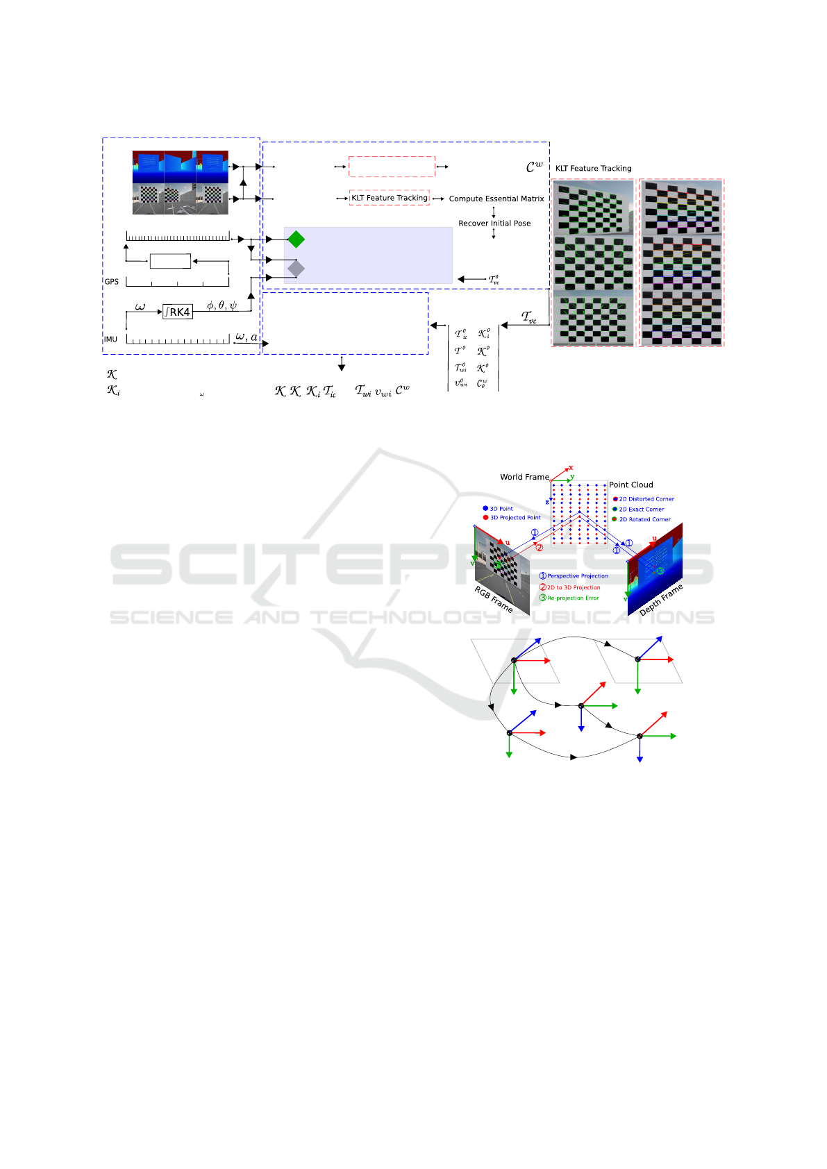
Figure 2: The pipeline of our method’s front-end and back-end. The front-end is an initial data processing layer after acquiring

RGB-D aligned frames. The back-end is the central processing layer of two optimization levels.

based RGB-D-IMU complete system calibration with

a novel depth correction model that does not require a

separate optimization stage to ﬁt the depth map on a

high-order parametric curve or surface. The robust-

ness of our method conforms to the works (Surber

et al., 2017; Bloesch et al., 2015), which can be

summed up in three main points: minimum infor-

mation is needed to efﬁciently bootstrap the system,

overcome inertial and celestial sensors limitations

during the initialization process, and efﬁcient mea-

surements outlier rejection (Antonante et al., 2021).

3 METHODOLOGY

This section presents a sequential overview of the pro-

posed calibration and pose estimation method. In

Section 3.1, we start by collecting the target’s poses

(up-to-scale) as well as the checkerboard corners and

construct an initial point cloud of the collected cor-

ners (see Figure 2 (top)). Then in Section 3.2, we

bootstrap the optimizer with GPS and gyroscope read-

ings for instant metric scale estimation of the esti-

mated target’s poses. Finally, Section 3.3 presents the

tightly-coupled hybridization factors to calibrate the

full RGB-D-IMU sensor setup in a non-linear BA op-

timization process.

3.1 Flow-Based Visual Odometry

Corners and their corresponding features from the

scene are ﬁrst extracted via (Shi and Tomasi, 1994)

with a block size of 17 pixels. To enhance the ro-

bustness and the versatility of the VO process, we

(a)

(b)

World (W)

IMU (I)

RGB (C)

Depth (D)

Visual (V)

Figure 3: Illustration for the re-projection error factors on

both RGB and Depth frames, as well as the coordinate

frames for all sensors undergoing optimization: (a) 3D to

2D and 2D to 3D to 2D re-projection error for triangulat-

ing the same target’s 3D corner on both the RGB-D current

aligned frames; (b) Coordinate frame of reference for all

sensors undergoing the calibration with respect to the world

frame. For consistency: all frames follow the right-handed

rule as OpenCV library.

adopt the optical ﬂow-based feature tracking method:

Kanade–Lucas–Tomasi (KLT) (Tomasi and Kanade,

1991), to match corresponding features in a pyramidal

resolution approach of 7 levels with a 17 × 17 pixels

window size.

On tracking the most robust and stable features

Robust RGB-D-IMU Calibration Method Applied to GPS-Aided Pose Estimation

PGO Factor

Range Factor

GPS reading

Gyroscope reading

KLT-VO Pose

RK4RK4 RK4RK4

CT-GPS

p(u)

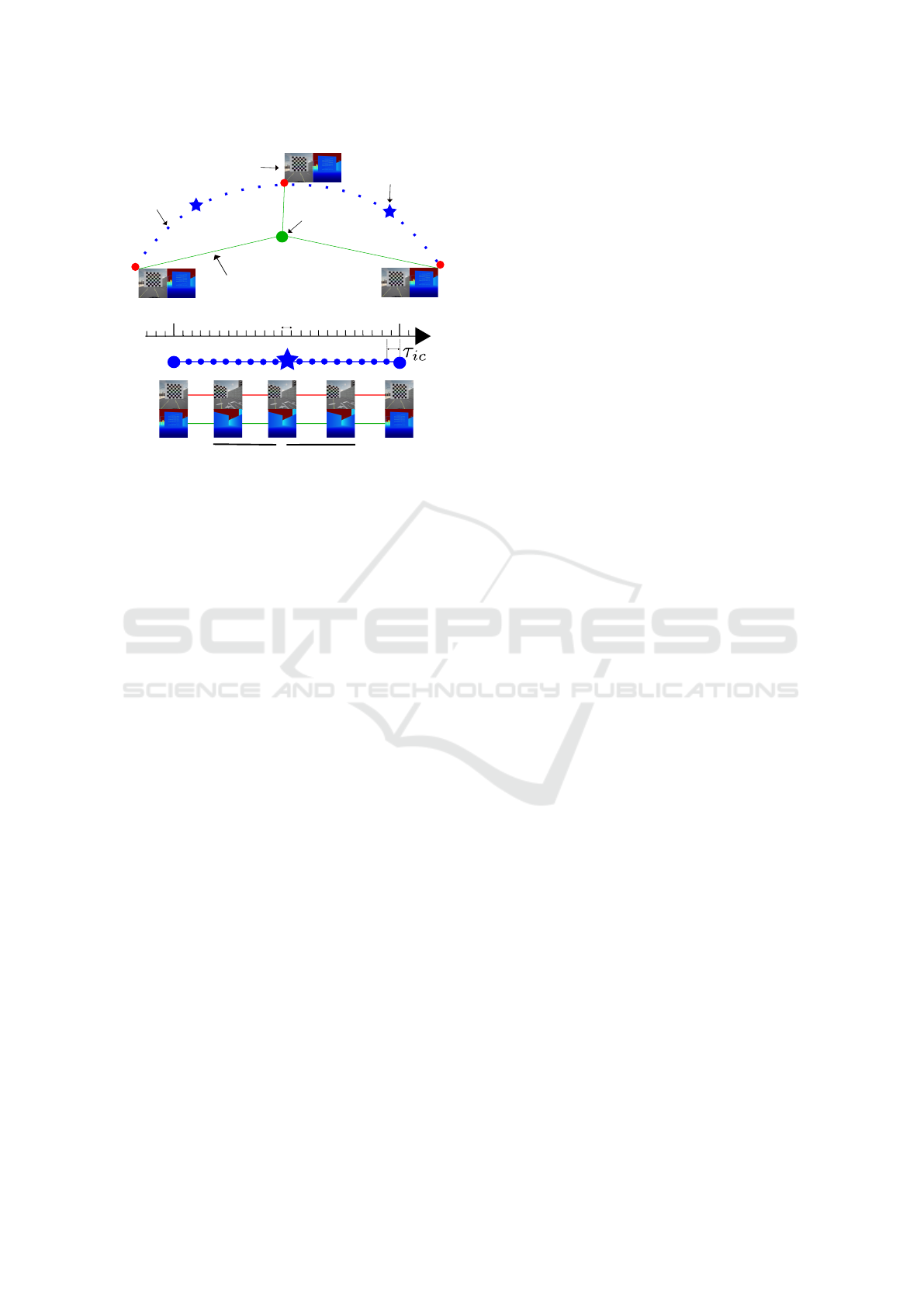
Figure 4: Level 1 factor graph. p(u) is the CT-GPS trajec-

tory generated at high frequency. RK4 is the Runge-Kutta

order gyroscope integration scheme. Dotted lines de-

note the error term (

−1

) in Equation (5) between any

two KLT-VO poses.

in 10 consecutive frames, we apply the 5-point algo-

rithm (Nist

er, 2004) to calculate the Essential Matrix

with feature outlier rejection by MAGSAC++ (Barath

et al., 2020), a more robust implementation of the

RANSAC method. Then the relative transformation

between every 2 consecutive frames T

∈ SE(3) is

recovered from the Essential Matrix, which we use to

initialize our level 1 optimization process with the ini-

tial pose graph using the following arbitrarily scaled

transformation:

˙= T

. T

, (1)

where T

∈ SE(3) is the rigid-body transforma-

tion between the IMU/body (world) and RGB camera

(visual) inertial frames of reference w, v, respectively.

In initialization, we assume that there is no transla-

tion between the IMU-camera reference frames, i.e.,

= [0, 0,0]

⊤

, and the rotation R

between them is

given in Figure 3 (b), knowing that the camera frame

c and its inertial frame of reference (visual frame v)

initially coincides on each other. Until this step, the

RGB camera’s rigid-body motion T

is considered

the arbitrary scaled rigid-body motion of all the multi-

modal sensor setup T

In parallel, a checkerboard corner detection is run

on all RGB camera frames. When a checkerboard is

detected, an RGB frame is considered a calibration

keyframe (KF). We integrate the corresponding time-

synchronized, and spatially aligned (Darwish et al.,

2017a) depth frame (d) to construct a 3D point cloud

of the currently detected corners.

3.2 Optimizer Robust Initialization

After obtaining the target’s poses and initially con-

structing point clouds of the checkerboard, bootstrap-

ping the optimizer is essential for a reliable calibra-

tion process. This method is efﬁcient in terms of com-

plexity since the bootstrapping relies only on low-

rate noisy GPS measurements and gyroscope prein-

tegrated readings. To tackle these GPS problems,

we apply an on-manifold cumulative B-spline inter-

polation (Sommer et al., 2020) to synthesize a very

smooth continuous-time (CT) trajectory ∈ R

from

the low-rate noisy GPS readings, as illustrated in Fig-

ure 4.

The matrix form for the cumulative B-spline man-

ifold of order k = n + 1, where n is the spline degree,

is modeled at t ∈ [t

i+k−1

] as:

p(u) = p

k−1

∑

j=1

(k)

. ¯u

(k)

∈ R

, (2)

where p(u) is the continuous-time B-spline increment

that interpolates k GPS measurements on the nor-

malized unit of time u(t) := (t − t

)/∆t

− P

where

1/∆t

denotes the spline generation frequency, P

the pose number that contributes to the current spline

segment P

∈ [0,··· ,k − 1]. p

is the initial discrete-

time (DT) GPS location measurement at time t

. d

i+ j

− p

i+ j−1

is the difference vector between two

consecutive DT-GPS readings.

(k)

is the cumulative

basis blending matrix and ¯u

(k)

is the normalized time

vector and are deﬁned as:

(k)

j,n

∑

k−1

s= j

(k)

s,n

(k)

s,n

k−1

(k−1)!

∑

k−1

l=s

(−1)

l−s

(k − 1 − l)

k−1−n

¯u

(k)

= [u

,·· · , u

k−1

, u

]

⊤

, u ∈ [0,· ·· , 1].

(3)

Our GPS-IMU-aided initialization system com-

prises two factors; the ﬁrst factor, r

, optimizes the 6-

DoF of every pose, whereas the second factor, r

, op-

timizes the positional 3-DoF between two poses with

a range constraint.

The level 1’s objective function L

p,s

is modeled as:

p,s

= argmin

∑

(i, j)



||r

(i, j)||

i, j

+ ||r

(i, j)||

i, j



(4)

i, j

,Σ

i, j

are the information matrices associated

with the GPS readings covariance, reﬂecting the

PGO and Range factors noises on the global metric

scale estimation process between two RGB-D aligned

frames.

Pose Graph Optimization (PGO) Factor. The PGO

is a 6-DoF factor that controls the relative pose error

between two consecutive edges i, j and is formulated

as:





−1



⊖ ∆T

ω,GPS

i j



, (5)

where ||.||

is the L2 norm,

i, j

∈ SE(3) is the T

estimated from the front-end pipeline at frames i, j.

VISAPP 2023 - 18th International Conference on Computer Vision Theory and Applications

RGB:

Depth:

IMU:

Δt

3D Point Cloud

Re-projection & Scale Factors

IMU Factors

IMU Measurements

{

NOT KF (No checkerboard detected)

keyframe

{

Figure 5: Level 2 factor graph between RGB-D aligned

keyframes (KF). This factor graph illustrates the non-linear

BA process to calibrate the full RGB-D-IMU sensor setup.

∆t denotes the IMU time step. τ

denotes the camera-IMU

time offset.

⊖ is the SE(3) logarithmic map as deﬁned in (Wang

and Chirikjian, 2008). ∆T

ω,GPS

i j

[δR

i j

,δp

GPS

i j

] ∈ se(3),

where δp

GPS

i j

= p

− p

is the CT-GPS measurement

increment and δR

i j

= [δφ,δθ, δψ] is the gyroscope in-

tegrated increment δR

i j

k=i

(ω

).dk using Runge-

Kutta 4

order (RK4) integration method (Zheng and

Zhang, 2017) between the two keyframes i, j.

Range Factor. The range factor limits the front-end

visual drift and keeps the global metric scale under

control within a sensible range deﬁned by the GPS

signal and is formulated as:



−

− ||p

GPS

− p

GPS



, (6)

where inner ||.||

is the Euclidean norm between the

translation vectors

i, j

, p

GPS

i, j

∈ R

of two consecutive

front-end (KLT-VO) poses and CT-GPS signals, re-

spectively.

3.3 RGB-D-IMU Local Bundle

Adjustment

To estimate the calibration parameters of the RGB-

D-IMU, we fuse the tracked checkerboard corners

and point clouds with the IMU preintegrated mea-

surements factor proposed in (Forster et al., 2016).

Figure 5 shows our sliding window approach. The

local BA is performed on all collected 2D corners

B within their corresponding 3D point cloud C be-

tween two aligned RGB camera c and Depth camera

d keyframes i, j, and the IMU readings I in-between.

Our local bundle-adjustment minimization objective

function L

c,d,I

is deﬁned by:

c,d,I

= argmin

∑

(i, j)

(||r

(i, j)||

i, j

)

∑



(||r

)||

) + ρ

(||r

)||

)

i

(7)

with X , the full local BA optimization states, which

is deﬁned as:

X =

{

}

= [ f

, f

, c

, k

, p

, k

, λ] ∈ R

= [τ

, b

] ∈ R

, ∀k ∈ [0, N],

= [R

, R

] ∈ SE(3),

= [X

, Y

, Z

] ∈ R

, ∀k ∈ [0, N],

(8)

where K

are intrinsic parameters containing the

cameras focal lengths f

, f

, focal centers c

, c

radial-tangential distortion coefﬁcients k

1,2,3

, p

1,2

and the cloud scale factor λ. T

are the inter-

sensor extrinsic rigid-body transformations. While

the spatio-temporal parameters include the scene

structure C

, the body metric scaled pose T

, veloc-

ity v

with respect to the world coordinates, τ

[sec]

is the IMU-camera time-offset (Voges and Wagner,

2018), and b

∈ R

, b

∈ R

are the gyroscope and

accelerometer biases, respectively. N,M are the

number of calibration keyframes and corner obser-

vations, respectively. r

are the IMU, corner

re-projection, and cloud-scale factors, respectively.

i, j

,Σ

are the information matrices associated

with the IMU readings I , detected corners B, and re-

constructed cloud C scale noise covariance. ρ is the

loss function deﬁned by Huber norm (Huber, 1992)

for r

and Cauchy norm (Black and Anandan,

1996) ρ

for r

Structured Re-Projection Errors Factor. We apply

the RGB camera pinhole model with radial-tangential

distortion coefﬁcients with intrinsic parameters ma-

trix K

. As illustrated in Figure 3 (a), we consider a

constructed 3D point cloud C

using the depth cam-

era aligned k

frame with the current RGB keyframe

k. For every checkerboard, we have H ×W feature ob-

servations, representing the keyframe’s detected cor-

ners B

[u,v].

There is a factor for every detected corner on the

current keyframe k that minimizes the error between

this corner’s location B

[u,v] and the re-projection of

the cloud’s C

(u,v) corresponding 3D point on k

Robust RGB-D-IMU Calibration Method Applied to GPS-Aided Pose Estimation

Figure 6: Illustration for the 2D-3D-2D projection of the

H ×W = 7 × 7 checkerboard feature points from the RGB

frame to the point cloud and then to the depth frame. λ is

the correction factor for RGB camera intrinsics to estimate

the cloud scale factor optimally.

keyframe after distortion

[ ˆu, ˆv]. This factor is de-

ﬁned by:

= ||B

[u,v] −

[ ˆu, ˆv]||

. (9)

Applying the pinhole camera radial-tangential dis-

tortion model (Zhang, 2000) to calculate the distorted

pixel location of the re-projected 3D point on the cur-

rent frame

[ ˆu, ˆv], we get:

(u,v) = T

−1

(u,v) = [X

¯u = X

+ c

/ f

, ¯v = Y

+ c

/ f

= ¯u

+ ¯v

ˆu = f

.( ¯u.(1 + k

+ k

+2.p

. ¯v)+ p

.(r

+ 2. ¯u

)),

ˆv = f

.( ¯v.(1 + k

+ k

+2.p

. ¯u) + p

.(r

+ 2. ¯v

)).

(10)

Cloud Scale Optimization Factor. This factor is

modeled to fuse the corner features from RGB frames

with the untextured depth maps to beneﬁt from the

advantages of both sensors by minimizing the error

between the distorted re-projection of the 3D cloud

point C

(u,v) on the k

depth frame

[ ˆu, ˆv] and the

current corner feature observation g

[u,v]) with

respect to it.

The effectiveness of this factor comes from the

hypothesis that undistorting the depth frame will, in

return, undistort the planar coordinates of the point

cloud C

]. In Figure 6, we apply the scale of

the cloud λ (known as inverse depth) to optimize the

RGB camera focal lengths with the cloud’s 3

coor-

dinate C

] which is optimized within the joint cal-

ibration model, knowing the metric scale of the pose.

This factor is deﬁned by:

= ||g

[u,v]) −

[ ˆu, ˆv]||

, (11)

where

[ ˆu, ˆv] follows the same model in Equa-

tion (10) by replacing C

(u,v) with C

(u,v) =

(u,v). g

(.) is a double re-projection with dis-

tortion function, that ﬁrstly projects the observation

[u,v] to the 3D point cloud C

[u,v]) as illus-

trated by red arrow numbered (2) in Figure 3 (a) using

the rigid-body transformation T

= T

from c to

w coordinates with the following formula:

[u,v]) = R

.(λ.K

−1

[u,v]) + t

. (12)

Then secondly, rotates C

[u,v]) to

[u,v]) using T

, and ﬁnally, re-projects

and undistorts this double rotated point on the depth

frame C

[u,v]) using the same model in Equation

(10).

IMU Factors. The IMU preintegration factors be-

tween two consecutive keyframes i, j is deﬁned in

(Forster et al., 2016) by:

= [∆R

i, j

,∆v

i, j

,∆p

i, j

,∆b

ω,a

i, j

] ∈ R

∆R

i, j

= log((∆

i, j

)

⊤

∆v

i, j

= R

⊤

.(v

− v

− g∆t

i, j

) − ∆ ˜v

i, j

∆p

i, j

= R

⊤

.(t

−t

− v

∆t

i, j

−

g∆t

i, j

) − ∆ ˜p

i, j

∆b

i, j

= ||b

− b

+ ||b

− b

(13)

where ∆

i, j

,∆ ˜v

i, j

,∆ ˜p

i, j

are the preintegrated rota-

tion, velocity and translation increments. All these

on-manifold preintegration increments derivations, as

well as the covariance Σ

i, j

propagation, are given in

the supplementary material of (Forster et al., 2016),

and for better readability, we write R

i, j

instead

of [R

4 EXPERIMENTS

We evaluate the performance of our method (see

Algorithm 1) on two applications: RGB-D-IMU

Calibration and GPS-aided pose estimation. Using

the IBISCape (Soliman et al., 2022) benchmark’s

CARLA-based data acquisition APIs, we collect three

simulated calibration sequences with a vast range of

sizes. Moreover, algorithm validation on simulated

sequences eases the change of settings to various sen-

sor conﬁgurations for robust validation of all corner

cases and provides a baseline for most system pa-

rameters. Furthermore, for real-world assessment, we

evaluate our calibration method on the RGB-D-IMU

checkerboard hand-eye calibration sequence from the

VCU-RVI benchmark (Zhang et al., 2020). Finally,

we conduct ablation studies on both IBISCape (Vehi-

cle) and EuRoC (Burri et al., 2016) (MAV) sequences

VISAPP 2023 - 18th International Conference on Computer Vision Theory and Applications

Algorithm 1: End-to-End Optimization Scheme.

Input: RGB frames (c), RGB-aligned depth

maps (d), GPS readings (DT-GPS), IMU readings (I )

Output: X =

{

}

1: T

⇐ KLT-VO (c, K

) ▷ Arbitrary scaled

2: T

⇐ rotate (T

∗ [T

]

−1

) ▷ Eq. (1)

3: B

[u,v] ⇐ collect corners (c, H, W) ▷ pix-2D

4: C

⇐ construct (d, B

[u,v], K

) ▷ Initial pcl-3D

5: p(u) ⇐ spline ﬁt (DT-GPS) ▷ Eq. (2)

6: [φ, θ,ψ] ⇐ RK4 (I

gyro

(ω)) ▷ Initial orientations

7: while not converged do ▷ Start Level 1

8: T

⇐ optimize (T

, p(u), [φ, θ,ψ]) ▷ Eq. (4)

9: end while

10: while not converged do ▷ Start Level 2

11: X ⇐ optimize (I , X

, C

)) ▷ Eq. (7)

12: end while

Table 1: Optimization process complexity analysis on IBIS-

Cape benchmark S1,S2,S3 sequences.

Level Initial Cost Final Cost Residuals Iterations Time

1.PGO

S1 1.69e+4 3.19e-9 2464 22 2.81”

S2 9.62e+4 3.12e-8 6951 26 8.79”

S3 1.47e+5 2.31e-8 14875 22 16.08”

Average 8097 23 9.23”

2.BA

S1 6.02e+7 1.57e+5 74820 274 2’40.56”

S2 3.67e+8 7.09e+5 210500 758 22’10.23”

S3 7.53e+8 1.22e+6 450696 779 49’22.04”

Average 245339 604 24’44.28”

to assess the contribution of each sensor in an RGB-

D-IMU-GPS setup to the accuracy of the pose estima-

tion for a reliable long-term navigation.

Factor graph optimization problems in Equations

(4) and (7) are modeled and solved using a sparse di-

rect method by the Ceres solver (Agarwal et al., 2022)

with the automatic differentiation tool for Jacobian

calculations. The sparse Schur linear method is ap-

plied to use the Schur complement for a more robust

and fast optimization process. Maximum calibration

time for the largest sequence S3 is ≈ 50[min] on a 16

cores 2.9 GHz processor and a Radeon NV166 RTX

graphics card. The front-end pipeline is developed in

Python for better visualization, and the back-end cost

functions are developed in C++ to decrease the sys-

tem latency during the optimization process.

A more in-depth quantitative analysis of the opti-

mization process computational cost is given in Table

1, where all experiments converged successfully. The

prominent conclusion from this complexity analysis

is that the level 2 BA optimization process is compu-

tationally highly expensive compared to the target’s

pose estimation optimization process of level 1. How-

ever, this level 2’s high computational load can still

compete with other calibration tools’ BA optimiza-

tion time, such as Kalibr (Rehder et al., 2016).

VCU-RVI (hand-eye)

Figure 7: The target’s top-view 3D point cloud recon-

struction; (left) VCU-RVI initially constructed point clouds,

(right) CARLA optimized point cloud. Blue dots with a red

outline denote the checkerboard corners 3D location. The

green colored curve represents the point cloud’s normal dis-

tribution convergence after optimization. Green circles de-

note a point cloud depth mean value.

4.1 Application I: RGB-D-IMU

Calibration

For both VCU-RVI and CARLA sequences, initial

values for the cameras’ intrinsic matrices are set to

W /2 for c

, f

, H/2 for c

, f

, and zeros for the radial-

tangential distortions. Initial λ is set with 0.1643,

which is the pixel density of CARLA cameras. For

extrinsic parameters T

and T

initialization, we set

the translation part with zeros, and the rotation matrix

is set as given in Figure 3 (b). Since the VCU-RVI

handheld sequence can provide sufﬁcient IMU exci-

tation but with no GPS data available, bootstrapping

the calibration system is performed by the traditional

IMU-based method (Qin et al., 2018).

We validate our new cloud global optimization

factor based on two criteria: the estimated point cloud

after optimization and the depth frame distortion esti-

mation as an indicator for depth correction. Figure 7

shows that the optimized cloud is converging to a nor-

mal distribution whose mean is the exact location in

the simulation world at 60 m which is at the checker-

board’s location as marked on Figure 8. Table 2 shows

the considerably high values for depth frame distor-

tion coefﬁcients, indicating our factor’s effect on the

cloud’s planar undistortion.

Using Kalibr (Rehder et al., 2016) as a baseline

for the RGB camera intrinsics for both CARLA and

VCU-RVI sequences, we evaluate our optimizer es-

timation quality in Table 2. Since the map scale λ

is an RGB camera optimization parameter based on

the RGB-D geometric linking constraint introduced in

Equation (12), the estimates of the focal length need

scale correction using: f

corr

x,y

= f

est

x,y

∗ λ. For the VCU-

RVI hand-eye sequence, we notice that the cloud scale

factor is approaching the value 1, which indicates

that the initial point cloud is constructed with a high-

Robust RGB-D-IMU Calibration Method Applied to GPS-Aided Pose Estimation

Table 2: RGB-D-IMU Sensors Setup Intrinsic Parameters Estimation. Since the CARLA simulator does not provide exact

intrinsics values, GT for RGB camera intrinsics are obtained with Kalibr (Rehder et al., 2016). KF: keyframes count. TL:

Sequence Trajectory Length. D: Sequence Duration.

∗

denotes a value calculated from the Structure Core (SC) RGB-D

camera speciﬁcations with depth FOV=70°.

∗∗

denotes a value from the Bosch BMI085 IMU technical data sheet.

Parameter

CARLA Simulator (IBISCape (Soliman et al., 2022)) VCU-RVI (Zhang et al., 2020)

S1 S2 S3 GT hand-eye GT

Speciﬁcations

RGB 20 Hz - 1024×1024 px 30 Hz - 640×480 px

Depth 20 Hz - 1024×1024 px 30 Hz - 640×480 px

IMU 6-axis acc/gyro @200Hz 6-axis acc/gyro @100Hz

#KF 353 994 2126 - 1118 -

TL[m] 122.06 345.42 737.88 - 11.16 -

D[sec] 17.640 49.730 106.29 - 46.59 -

RGB Camera

λ. f

164.01 122.71 148.42 151.51 375.67 459.36

λ. f

163.30 122.22 149.39 151.89 398.44 459.76

498.89 506.21 507.59 510.01 315.48 332.69

514.01 515.49 518.61 510.71 289.64 258.99

-5.10e-3 -6.20e-3 -6.15e-3 2.42e-5 -1.62e-2 -2.98e-1

-1.95e-3 -1.96e-3 -2.07e-3 2.89e-6 -3.62e-3 9.22e-2

-1.25e-3 -1.96e-3 -8.31e-4 1.71e-4 -2.31e-3 -1.19e-4

-3.20e-3 -2.27e-3 -3.53e-3 -3.22e-5 -1.09e-2 -7.46e-5

-8.16e-4 -8.70e-4 -8.64e-4 0.0 -7.84e-4 -

λ 0.3581 0.2819 0.3432 - 0.9831 -

Depth Camera

511.42 511.51 511.51 512.0 456.82 457.01

∗

511.91 511.83 511.82 512.0 456.06 457.01

∗

512.20 512.22 512.30 512.0 333.29 320.0

∗

511.81 512.01 512.02 512.0 259.17 240.0

∗

-3.53e-2 -3.37e-2 -3.54e-2 - -5.74e-2 -

-5.60e-3 -6.20e-3 -6.25e-3 - -9.07e-3 -

-3.41e-2 -3.22e-2 -3.29e-2 - -4.13e-2 -

-3.93e-2 -3.50e-2 -3.82e-2 - -6.09e-2 -

-1.10e-3 -1.45e-3 -1.38e-3 - -2.98e-4 -

IMU Sensor

4.986e-3 4.989e-3 4.998e-3 5e-3 4.473e-3 -

-7.549e-3 -2.242e-2 -4.907e-3 -2.383e-3 1.512e-4 9.69e-5

∗∗

-3.283e-2 3.813e-2 -2.054e-2 -3.364e-3 9.337e-5 9.69e-5

∗∗

8.151e-2 2.659e-2 -2.540e-2 1.555e-3 -2.967e-4 9.69e-5

∗∗

0.109 -0.062 0.147 -0.951 -5.704e-4 -

-0.707 -1.069 -0.091 -0.691 6.757e-4 -

-1.926 -2.295 -2.364 0.183 -9.304e-4 -

Table 3: Extrinsic parameters estimation for both IBISCape (S1,S2,S3) and VCU-RVI (hand-eye) calibration sequences.

Parameter t

[m] t

[m] q

RGB-D (T

)

S1 4.95e-3 0.017 0.037 -0.037 -0.022 0.030 0.997

S2 5.47e-3 0.020 0.065 -0.041 0.005 0.019 0.996

S3 9.10e-3 0.018 0.065 -0.036 -0.010 0.025 0.997

GT 0.0 0.020 0.060 0.0 0.0 0.0 1.0

hand-eye -0.103 0.003 0.018 0.041 0.081 0.009 0.969

GT -0.100 0.0 0.0 0.0 0.0 0.0 1.0

RGB-IMU (T

)

S1 -0.806 0.154 -0.308 0.493 0.507 0.499 0.500

S2 -0.854 -0.057 0.006 0.503 0.495 0.501 0.498

S3 -0.808 -0.028 -0.102 0.503 0.501 0.499 0.496

GT -0.800 0.0 0.0 0.500 0.500 0.500 0.500

hand-eye 0.077 0.020 -0.041 0.699 -0.713 -0.009 -9e-4

GT -0.008 0.015 -0.011 0.708 -0.706 0.001 -4e-4

Table 4: Ablation study on the contribution of the GPS sensor on the system accuracy when depth information is available.

Method

IBISCape (Soliman et al., 2022) (RPE

(µ ± σ) [m])

Average

S1 S2 S3

DUI-VIO (Zhang and Ye, 2020) 0.115±0.113 0.115±0.114 0.120±0.119 0.117±0.115

BASALT (Usenko et al., 2019) 0.084±0.084 0.052±0.051 0.026±0.026 0.054±0.054

ORB-SLAM3 (Campos et al., 2021) 0.028±0.013 0.073±0.034 0.031±0.028 0.044±0.025

Proposed (Lvl.1+2) 0.016±0.019 0.025±0.030 0.018±0.025 0.020±0.025

VISAPP 2023 - 18th International Conference on Computer Vision Theory and Applications

Proposed (Lvl.1+2)

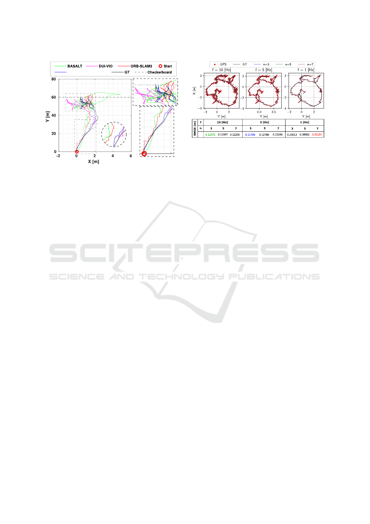
Figure 8: Pose estimation evaluation of our method com-

pared to ORB-SLAM3, BASALT, and DUI-VIO on S1 se-

quence. Different axes scale for showing ﬁne details.

quality depth sensor.

In Table 3, we show the optimal performance of

our optimizer to estimate the inter-sensor extrinsic pa-

rameters compared to the GT values. Compared to the

baseline, our optimizer efﬁciently estimates the inter-

sensor rotation and translation in the case of RGB-

D sensors. For the IMU-camera extrinsic parameters

and in contrast to rotations, the IMU-camera rigid-

body translation mainly depends on the initial values

set in the optimizer. In order to estimate the optimal

values for the translation part, multiple experiments

should be executed with zeros as initial conditions

with large data sets. Based on the quality of the IMU

still calibration values, all the experiments will con-

verge to relative values, as shown in Table 3.

4.2 Application II: GPS-Aided Pose

Estimation

Two ablation studies are carried out to assess the con-

tribution of the GPS sensor to the accuracy of the

pose estimation when the depth information is avail-

able or not available. Standard VIO evaluation met-

rics (Chen et al., 2022) are used for assessment: Root

Mean Square Absolute Trajectory Error (RMS ATE

[m]) and Relative Pose Error (RPE

[m]).

4.2.1 Ablation Study on a Simulated Ground

Vehicle

In the ﬁrst ablation study, we assess the performance

of our depth-incorporated pose estimation with GPS-

aided bootstrapping compared to the latest state-of-

the-art VIO systems that do not utilize GPS read-

ings in their estimations. We compare our GPS-

aided RGB-D-IMU pose estimation accuracy with

Figure 9: Synthesizing low-rate noisy DT-GPS readings

with three frequencies [10,5,1] Hz on EuRoC V2-01 se-

quence and performing the B-spline interpolation (CT-GPS)

with manifolds of degree (n=3,5,7). Blue denotes the most

accurate, red denotes the least accurate, and green denotes

the parameters used in our experiments (n=3, f=10Hz).

RMSE is the accuracy evaluation metric.

that of ORB-SLAM3 (RGB-D) (Campos et al., 2021),

BASALT (2×RGB-IMU) (Usenko et al., 2019), and

DUI-VIO (RGB-D-IMU) (Zhang and Ye, 2020) sys-

tems using both VCU-RVI and CARLA sequences.

During the evaluation of the DUI-VIO (Zhang and

Ye, 2020) system, we noticed an initialization failure

with the S1 sequence till the system initialized suc-

cessfully at the end of the speed bump at nearly 30

m as magniﬁed in Figure 8 (#1). This initialization

problem is not witnessed with the VCU-RVI hand-

eye calibration sequence due to its complex combined

motions (see Figure 1 (right)). Sequences (S2, S3)

are simulated with a high combined motion to ensure

the optimal checkerboard coverage for all the RGB-D

camera frames. The complex motion generated sufﬁ-

cient IMU excitation to initialize BASALT and DUI-

VIO.

In our analysis in Table 4, the quantitative results

show superior performance for our method compared

to other approaches. Indeed, the pose estimation error

is reduced by 54.55%, 62.96%, and 82.91% compared

to ORB-SLAM3, BASALT, and DUI-VIO, respec-

tively. This happens thanks to our fast bootstrapping

GPS-aided method that decreases the relative pose er-

ror accumulation with time.

4.2.2 Ablation Study on a Real-World Aerial

Vehicle

To further validate the performance of our pose es-

timation method in a real-world application, we per-

form another ablation study. The experiments of this

study were performed on the EuRoC MAV dataset

(Burri et al., 2016) incorporating RGB-IMU sensors

and compared to the continuous-time and discrete-

time (CT/DT) GPS-based SLAM system proposed in

Robust RGB-D-IMU Calibration Method Applied to GPS-Aided Pose Estimation

Table 5: Ablation study on the contribution of the GPS sensor on the system accuracy when depth information is unavailable.

∗

denotes tracking features in 5 consecutive frames instead of 10 due to the rapid motion of the MAV.

denotes the only

learning-based baseline in the table and the only method incorporating LiDAR point clouds. V,I,G: Vision, IMU, and GPS.

Method

EuRoC (Burri et al., 2016) (RMS ATE

[m])

Avg.

V1-01 V1-02 V1-03 V2-01 V2-02 V2-03

Mono-VI

OKVIS (Leutenegger et al., 2015) 0.090 0.200 0.240 0.130 0.160 0.290 0.185

ROVIO (Bloesch et al., 2015) 0.100 0.100 0.140 0.120 0.140 0.140 0.123

VINS-Mono (Qin et al., 2018) 0.047 0.066 0.180 0.056 0.090 0.244 0.114

OpenVINS (Geneva et al., 2020) 0.056 0.072 0.069 0.098 0.061 0.286 0.107

CodeVIO

(Zuo et al., 2021) 0.054 0.071 0.068 0.097 0.061 0.275 0.104

Stereo-VI

VINS-Fusion (Qin et al., 2019) 0.076 0.069 0.114 0.066 0.091 0.096 0.085

BASALT (Usenko et al., 2019) 0.040 0.020 0.030 0.030 0.020 0.050 0.032

Kimera (Rosinol et al., 2020) 0.050 0.110 0.120 0.070 0.100 0.190 0.107

ORB-SLAM3 (Campos et al., 2021) 0.038 0.014 0.024 0.032 0.014 0.024 0.024

Mono-V/I/G

CT (V+I+G) (Ciofﬁ et al., 2022) 0.024 0.014 0.011 0.012 0.010 0.010 0.014

CT (V+G) (Ciofﬁ et al., 2022) 0.011 0.013 0.012 0.009 0.008 0.012 0.011

CT (I+G) (Ciofﬁ et al., 2022) 0.062 0.102 0.117 0.112 0.164 0.363 0.153

DT (V+I+G) (Ciofﬁ et al., 2022) 0.016 0.024 0.018 0.009 0.018 0.033 0.020

DT (V+G) (Ciofﬁ et al., 2022) 0.010 0.025 0.024 0.010 0.012 0.029 0.018

DT (I+G) (Ciofﬁ et al., 2022) 0.139 0.137 0.138 0.138 0.138 0.139 0.138

Proposed (Lvl.1) 0.008 0.017

∗

0.023

∗

0.008 0.022 0.025

∗

0.017

(Ciofﬁ et al., 2022). Since a comparison with the

competing technique (Ciofﬁ et al., 2022), combining

GPS signals computed from the Vicon system mea-

surements better emphasizes the ﬁndings of this abla-

tion research, we chose the identical six Vicon room

sequences from the EuRoC benchmark they used in

their evaluation.

The GPS readings for EuRoC sequences are gen-

erated with the same realistic model and parameters

given in (Ciofﬁ et al., 2022) that gives a real-world

accuracy but does not suffer from limitations as mul-

tipath effects (Obst et al., 2012). CARLA GPS sensor

is modeled as most commercial sensors containing a

particular bias with a random noise seed and a zero

mean Gaussian noise added to every reading. The

most prominent conclusion from Figure 9 is that as

the GPS rate increases, the CT-GPS interpolation is

better with a low degree (n) manifold, and vice-versa,

and our GPS-aided initialization method can still be

valid with the lowest GPS frequency ( f = 1 Hz).

The quantitative analysis in Table 5 shows that

our level 1 estimations, with no depth information,

can efﬁciently estimate a metric-scaled trajectory that

can bootstrap level 2 and outperform other well-

established VIO systems in terms of accuracy. We

also notice an improvement in estimation accuracy

with adding a sensor modality (IMU/GPS), given that

at least one visual sensor is present in the system. An-

other conclusion is that a GPS can be sufﬁcient with

the optical sensor to get a reliable trajectory estimate

in a tightly-coupled fusion scheme. For a loosely-

coupled fusion scheme (proposed Lvl.1), adding a gy-

roscope increases the conﬁdence of the optimizer to

converge to reasonable values.

5 CONCLUSION

This paper proposes the ﬁrst baseline method for ro-

bust RGB-D-IMU intrinsic and extrinsic calibration.

We ﬁrst present an RGB-GPS-Gyro optimizer boot-

strapping approach that estimates metric-scaled tar-

get’s pose reliable for the calibration process. Then,

we deﬁne a cloud-scale factor for an RGB-D spatially

aligned untextured depth map that estimates its scale

by incorporating the initially reconstructed cloud’s

uncertainty.

Experimental results on real-world and simulated

sequences show the effectiveness of our method. That

gives the main conclusion that it can be considered

the building block of a novel RGB-D GPS-aided VI-

SLAM system with a reliable online calibration al-

gorithm. In future work, it is indispensable to incor-

porate situations where GPS sensor limitations cannot

be simulated as the multipath effects on the optimizer.

Finally, it will be essential to generalize the BA op-

timization problem further to extend the algorithm’s

calibration capability to include multiple IMUs with

multiple vision sensors (RGB and depth).

VISAPP 2023 - 18th International Conference on Computer Vision Theory and Applications

REFERENCES

Agarwal, S., Mierle, K., and Team, T. C. S. (2022). Ceres

Solver.

Antonante, P., Tzoumas, V., Yang, H., and Carlone, L.

(2021). Outlier-robust estimation: Hardness, min-

imally tuned algorithms, and applications. IEEE

Transactions on Robotics, 38(1):281–301.

Barath, D., Noskova, J., Ivashechkin, M., and Matas, J.

(2020). MAGSAC++, a fast, reliable and accurate ro-

bust estimator. In Proceedings of the IEEE/CVF Con-

ference on Computer Vision and Pattern Recognition

(CVPR).

Basso, F., Menegatti, E., and Pretto, A. (2018). Robust in-

trinsic and extrinsic calibration of RGB-D cameras.

IEEE Transactions on Robotics, 34(5):1315–1332.

Black, M. J. and Anandan, P. (1996). The Robust Estima-

tion of Multiple Motions: Parametric and Piecewise-

Smooth Flow Fields. Computer Vision and Image Un-

derstanding, 63(1):75–104.

Bloesch, M., Omari, S., Hutter, M., and Siegwart, R.

(2015). Robust visual inertial odometry using a di-

rect EKF-based approach. In 2015 IEEE/RSJ Interna-

tional Conference on Intelligent Robots and Systems

(IROS), pages 298–304.

Brunetto, N., Salti, S., Fioraio, N., Cavallari, T., and Ste-

fano, L. (2015). Fusion of inertial and visual mea-

surements for RGB-D slam on mobile devices. In

Proceedings of the IEEE International Conference on

Computer Vision Workshops, pages 1–9.

Burri, M., Nikolic, J., Gohl, P., Schneider, T., Rehder, J.,

Omari, S., Achtelik, M. W., and Siegwart, R. (2016).

The EuRoC micro aerial vehicle datasets. The Inter-

national Journal of Robotics Research, 35(10):1157–

1163.

Campos, C., Elvira, R., Rodr

ıguez, J. J. G., Montiel, J. M.,

and Tard

os, J. D. (2021). OrbSLAM3: An accu-

rate open-source library for visual, visual–inertial,

and multimap slam. IEEE Transactions on Robotics,

37(6):1874–1890.

Chai, W., Chen, C., and Edwan, E. (2015). Enhanced indoor

navigation using fusion of IMU and RGB-D camera.

In International Conference on Computer Information

Systems and Industrial Applications, pages 547–549.

Atlantis Press.

Chang, Z., Meng, Y., Liu, W., Zhu, H., and Wang, L. (2022).

WiCapose: multi-modal fusion based transparent au-

thentication in mobile environments. Journal of Infor-

mation Security and Applications, 66:103130.

Chen, W., Shang, G., Ji, A., Zhou, C., Wang, X., Xu, C.,

Li, Z., and Hu, K. (2022). An Overview on Visual

SLAM: From Tradition to Semantic. Remote Sensing,

14(13).

Chghaf, M., Rodriguez, S., and Ouardi, A. E. (2022). Cam-

era, LiDAR and multi-modal SLAM systems for au-

tonomous ground vehicles: a survey. Journal of Intel-

ligent & Robotic Systems, 105(1):1–35.

Chow, J. C., Lichti, D. D., Hol, J. D., Bellusci, G., and

Luinge, H. (2014). IMU and multiple RGB-D camera

fusion for assisting indoor stop-and-go 3D terrestrial

laser scanning. Robotics, 3(3):247–280.

Chu, C. and Yang, S. (2020). Keyframe-based RGB-D

visual-inertial odometry and camera extrinsic calibra-

tion using Extended Kalman Filter. IEEE Sensors

Journal, 20(11):6130–6138.

Ciofﬁ, G., Cieslewski, T., and Scaramuzza, D. (2022).

Continuous-time vs. discrete-time vision-based

SLAM: A comparative study. IEEE Robotics Autom.

Lett., 7(2):2399–2406.

Darwish, W., Li, W., Tang, S., and Chen, W. (2017a).

Coarse to ﬁne global RGB-D frames registration for

precise indoor 3D model reconstruction. In 2017

International Conference on Localization and GNSS

(ICL-GNSS), pages 1–5. IEEE.

Darwish, W., Tang, S., Li, W., and Chen, W. (2017b). A

new calibration method for commercial RGB-D sen-

sors. Sensors, 17(6):1204.

Das, A., Elfring, J., and Dubbelman, G. (2021). Real-

time vehicle positioning and mapping using graph op-

timization. Sensors, 21(8):2815.

Forster, C., Carlone, L., Dellaert, F., and Scaramuzza,

D. (2016). On-manifold preintegration for real-

time visual–inertial odometry. IEEE Transactions on

Robotics, 33(1):1–21.

Geneva, P., Eckenhoff, K., Lee, W., Yang, Y., and Huang,

G. (2020). OpenVINS: a research platform for visual-

inertial estimation. In 2020 IEEE International Con-

ference on Robotics and Automation (ICRA), pages

4666–4672.

Guo, C. X. and Roumeliotis, S. I. (2013). IMU-RGBD cam-

era 3D pose estimation and extrinsic calibration: Ob-

servability analysis and consistency improvement. In

2013 IEEE International Conference on Robotics and

Automation, pages 2935–2942. IEEE.

Heyden, A. and Pollefeys, M. (2005). Multiple view geom-

etry. Emerging topics in computer vision, 90:180–189.

Huai, J., Zhuang, Y., Lin, Y., Jozkow, G., Yuan, Q., and

Chen, D. (2022). Continuous-time spatiotemporal

calibration of a rolling shutter camera-IMU system.

IEEE Sensors Journal, 22(8):7920–7930.

Huber, P. J. (1992). Robust estimation of a location param-

eter. In Breakthroughs in statistics, pages 492–518.

Springer.

Hug, D., Banninger, P., Alzugaray, I., and Chli, M.

(2022). Continuous-time stereo-inertial odometry.

IEEE Robotics and Automation Letters, pages 1–1.

Jung, K., Shin, S., and Myung, H. (2022). U-VIO: Tightly

Coupled UWB Visual Inertial Odometry for Robust

Localization. In International Conference on Robot

Intelligence Technology and Applications, pages 272–

283. Springer.

Laidlow, T., Bloesch, M., Li, W., and Leutenegger, S.

(2017). Dense RGB-D-inertial SLAM with map de-

formations. In 2017 IEEE/RSJ International Confer-

ence on Intelligent Robots and Systems (IROS), pages

6741–6748. IEEE.

Lee, J., Hanley, D., and Bretl, T. (2022). Extrinsic calibra-

tion of multiple inertial sensors from arbitrary trajec-

tories. IEEE Robotics and Automation Letters.

Robust RGB-D-IMU Calibration Method Applied to GPS-Aided Pose Estimation

Leutenegger, S., Lynen, S., Bosse, M., Siegwart, R., and

Furgale, P. (2015). Keyframe-based visual–inertial

odometry using nonlinear optimization. The Interna-

tional Journal of Robotics Research, 34(3):314–334.

Ling, Y., Liu, H., Zhu, X., Jiang, J., and Liang, B.

(2018). RGB-D inertial odometry for indoor robot

via Keyframe-based nonlinear optimization. In 2018

IEEE International Conference on Mechatronics and

Automation (ICMA), pages 973–979. IEEE.

Liu, H., Qu, D., Xu, F., Zou, F., Song, J., and Jia, K. (2020).

Approach for accurate calibration of RGB-D cameras

using spheres. Opt. Express, 28(13):19058–19073.

Nist

er, D. (2004). An efﬁcient solution to the ﬁve-point

relative pose problem. IEEE transactions on pattern

analysis and machine intelligence, 26(6):756–770.

Obst, M., Bauer, S., Reisdorf, P., and Wanielik, G. (2012).

Multipath detection with 3D digital maps for robust

multi-constellation gnss/ins vehicle localization in ur-

ban areas. In 2012 IEEE Intelligent Vehicles Sympo-

sium, pages 184–190.

Ovr

en, H., Forss

en, P.-E., and T

ornqvist, D. (2013). Why

would I want a gyroscope on my RGB-D sensor? In

2013 IEEE Workshop on Robot Vision (WORV), pages

68–75. IEEE.

Qin, T., Li, P., and Shen, S. (2018). VINS-Mono: a robust

and versatile monocular visual-inertial state estimator.

IEEE Transactions on Robotics, 34(4):1004–1020.

Qin, T., Pan, J., Cao, S., and Shen, S. (2019). A gen-

eral optimization-based framework for local odome-

try estimation with multiple sensors. arXiv preprint

arXiv:1901.03638.

Rehder, J., Nikolic, J., Schneider, T., Hinzmann, T., and

Siegwart, R. (2016). Extending kalibr: Calibrating the

extrinsics of multiple IMUs and of individual axes. In

2016 IEEE International Conference on Robotics and

Automation (ICRA), pages 4304–4311. IEEE.

Rosinol, A., Abate, M., Chang, Y., and Carlone, L. (2020).

Kimera: an open-source library for real-time metric-

semantic localization and mapping. In 2020 IEEE In-

ternational Conference on Robotics and Automation

(ICRA), pages 1689–1696. IEEE.

Shan, Z., Li, R., and Schwertfeger, S. (2019). RGBD-

inertial trajectory estimation and mapping for ground

robots. Sensors, 19(10):2251.

Shi, J. and Tomasi (1994). Good features to track. In 1994

Proceedings of IEEE Conference on Computer Vision

and Pattern Recognition, pages 593–600.

Soliman, A., Bonardi, F., Sidib

e, D., and Bouchafa, S.

(2022). IBISCape: A simulated benchmark for multi-

modal SLAM systems evaluation in large-scale dy-

namic environments. Journal of Intelligent & Robotic

Systems, 106(3):53.

Sommer, C., Usenko, V., Schubert, D., Demmel, N., and

Cremers, D. (2020). Efﬁcient derivative computa-

tion for cumulative b-splines on lie groups. In 2020

IEEE/CVF Conference on Computer Vision and Pat-

tern Recognition, CVPR 2020, Seattle, WA, USA, June

13-19, 2020, pages 11145–11153. IEEE.

Staranowicz, A., Brown, G. R., Morbidi, F., and Mariottini,

G. L. (2014). Easy-to-Use and accurate calibration of

RGB-D cameras from spheres. In Klette, R., Rivera,

M., and Satoh, S., editors, Image and Video Tech-

nology, pages 265–278, Berlin, Heidelberg. Springer

Berlin Heidelberg.

Surber, J., Teixeira, L., and Chli, M. (2017). Robust visual-

inertial localization with weak GPS priors for repet-

itive UAV ﬂights. In 2017 IEEE International Con-

ference on Robotics and Automation (ICRA), pages

6300–6306.

Tomasi, C. and Kanade, T. (1991). Detection and tracking

of point. Int J Comput Vis, 9:137–154.

Usenko, V., Demmel, N., Schubert, D., St

uckler, J., and

Cremers, D. (2019). Visual-inertial mapping with

non-linear factor recovery. IEEE Robotics and Au-

tomation Letters, 5(2):422–429.

Voges, R. and Wagner, B. (2018). Timestamp offset cali-

bration for an IMU-Camera system under interval un-

certainty. In 2018 IEEE/RSJ International Conference

on Intelligent Robots and Systems (IROS), pages 377–

384.

Wang, Y. and Chirikjian, G. S. (2008). Nonparametric

second-order theory of error propagation on motion

groups. The International journal of robotics re-

search, 27(11-12):1258–1273.

Xiao, X., Zhang, Y., Li, H., Wang, H., and Li, B. (2022).

Camera-IMU Extrinsic Calibration Quality Monitor-

ing for Autonomous Ground Vehicles. IEEE Robotics

and Automation Letters, 7(2):4614–4621.

Zhang, H., Jin, L., and Ye, C. (2020). The VCU-RVI Bench-

mark: Evaluating Visual Inertial Odometry for Indoor

Navigation Applications with an RGB-D Camera. In

2020 IEEE/RSJ International Conference on Intelli-

gent Robots and Systems (IROS), pages 6209–6214.

Zhang, H. and Ye, C. (2020). DUI-VIO: Depth uncer-

tainty incorporated visual inertial odometry based on

an RGB-D camera. In 2020 IEEE/RSJ International

Conference on Intelligent Robots and Systems (IROS),

pages 5002–5008. IEEE.

Zhang, Y., Liang, W., Zhang, S., Yuan, X., Xia, X., Tan,

J., and Pang, Z. (2022). High-precision Calibra-

tion of Camera and IMU on Manipulator for Bio-

inspired Robotic System. Journal of Bionic Engineer-

ing, 19(2):299–313.

Zhang, Z. (2000). A ﬂexible new technique for camera cal-

ibration. IEEE Transactions on Pattern Analysis and

Machine Intelligence, 22(11):1330–1334.

Zheng, L. and Zhang, X. (2017). Chapter 8 - numerical

methods. In Zheng, L. and Zhang, X., editors, Mod-

eling and Analysis of Modern Fluid Problems, Math-

ematics in Science and Engineering, pages 361–455.

Academic Press.

Zhou, Y., Chen, D., Wu, J., Huang, M., and Weng, Y.

(2022). Calibration of RGB-D camera using depth

correction model. Journal of Physics: Conference Se-

ries, 2203(1):012032.

Zuo, X., Merrill, N., Li, W., Liu, Y., Pollefeys, M., and

Huang, G. P. (2021). CodeVIO: visual-inertial odom-

etry with learned optimizable dense depth. 2021 IEEE

International Conference on Robotics and Automation

(ICRA), pages 14382–14388.

VISAPP 2023 - 18th International Conference on Computer Vision Theory and Applications