Accurate Cutting of MSDM-Based Hybrid Surface Meshes

Thomas Kniplitsch

1 a

, Wolfgang Fenz

1 b

and Christoph Anthes

2 c

RISC Software GmbH, Softwarepark 32a, 4232 Hagenberg, Austria

University of Applied Sciences Upper Austria, Campus Hagenberg, Softwarepark 11, 4232 Hagenberg, Austria

Keywords:

Hybrid Mesh, Mass-Spring-Damper Model, Space Partitioning, Surface Mesh Cutting, Point Clustering.

Abstract:

The mass-spring-damper model (MSDM) is a popular method for the physics simulation of surface meshes.

Cutting such meshes requires consideration of various contradicting factors: accurate cut representation, main-

taining material properties (given by the MSDM geometry) and simulation cost. A hybrid mesh approach par-

tially decouples physics simulation mesh from render mesh by allowing partially rendered physics simulation

elements. This paper presents a cutting method for hybrid surface meshes which provides accurate cut repre-

sentation and maintains MSDM element geometry of cut areas while keeping simulation costs at a competitive

level. Additionally, auxiliary data structures, suitable for independent usage, are presented. The bounding box

ternary tree is a space partitioning data structure for storing volumetric objects. It subdivides space along an

axis-aligned separation plane at each tree level, partitioning objects into below, above and intersecting. A point

clustering data structure for efﬁcient retrieval of all points within a given distance is also presented.

1 INTRODUCTION

Surface meshes are a suitable representation for ob-

jects of uniform thickness with a large surface area

compared to their volume, e.g. cloth or membranes.

The MSDM and the ﬁnite element method are com-

monly used methods for the realtime simulation of

such structures. Compared to the ﬁnite element

method, the MSDM’s graph structure is relatively

simple, computationally cheap and allows to add/re-

move nodes and edges during runtime. This feature

is especially useful when the simulated mesh is cut,

which requires respective adaptations in the MSDM

mesh. Existing cutting methods compromise between

• the accuracy with which a cut is represented in the

rendered mesh,

• maintaining the material properties by preserving

the MSDM mesh geometry and

• the costs of the physics simulation which results

from the number of simulated elements.

As cut accuracy depends on the respective subdivi-

sion of the render mesh and material properties on the

preservation of MSDM element geometry, it is desir-

able to achieve both by decoupling these representa-

tions via a hybrid mesh approach.

https://orcid.org/0000-0002-3290-9345

https://orcid.org/0000-0002-6143-3024

https://orcid.org/0000-0002-0878-874X

The cutting algorithm presented in this paper uses

the hybrid mesh approach to duplicate cut-through

physics simulation triangles and divide the respective

render area among the copies. MSDM element ge-

ometry is therefore preserved and its element size de-

coupled from the precision with which cuts are repre-

sented on the surface area of the mesh. This allows for

potentially larger physics triangles, which can be de-

sirable, as fewer elements are needed to cover a given

simulation area and forces are propagated faster over

a ﬁxed distance. Deformations are also proportion-

ally smaller on larger elements, leading to less ex-

treme reactions and a more stable simulation. The

algorithm also incorporates methods to minimize the

number of newly created render mesh elements using

various merge distances.

Auxiliary data structures for space partitioning

and point clustering were developed. A bounding box

ternary tree (BBTT) uses axis-aligned planes to re-

cursively subdivide space and store elements below/

above/intersecting the plane in respective subtrees. A

point cluster dictionary (PCD) is used for merging

points within a speciﬁed merge distance δ

, storing

cluster centers depending on their position in a δ

based grid. In this paper “bounding box (BB)” always

refers to an “axis-aligned BB”.

These data structures, as well as the cutting al-

gorithm, have to account for ﬂoating point errors.

Whenever ﬂoating point numbers are handled, this

188

Kniplitsch, T., Fenz, W. and Anthes, C.

Accurate Cutting of MSDM-Based Hybrid Surface Meshes.

DOI: 10.5220/0011656200003417

In Proceedings of the 18th International Joint Conference on Computer Vision, Imaging and Computer Graphics Theory and Applications (VISIGRAPP 2023) - Volume 1: GRAPP, pages

188-195

ISBN: 978-989-758-634-7; ISSN: 2184-4321

 2023 by SCITEPRESS – Science and Technology Publications, Lda. Under CC license (CC BY-NC-ND 4.0)

paper assumes the maximum ﬂoating point error is

capped by a value δ

The paper is structured as follows: In Section 2

existing cutting methods and related work are pre-

sented. Section 3 introduces the MSDM and the hy-

brid mesh structure used for the cutting algorithm pre-

sented in Section 4. Auxiliary data structures for the

algorithm are described in Section 5, the algorithm’s

test results in Section 6. The paper concludes in Sec-

tion 7, where it also presents future work.

The main contribution of this paper is the pre-

sented cutting algorithm, whose algorithmic steps are

described in detail. Compared to other methods for

hybrid surface meshes (Molino et al., 2004; Wang

et al., 2014), element subdivision and accuracy of

cut representation is only limited by merge distances

which themselves have a lower bound of δ

2 RELATED WORK

Wu et al. provide an exhaustive review of cutting

methods and deformation models (Wu et al., 2015).

For triangular surface meshes the following cutting

methods, partially derived from tetrahedral cutting

methods, are presented:

• Element deletion removes cut triangles from the

mesh (Cotin et al., 2000).

• Splitting along existing faces moves the cutting

line to the closest triangle edge (Nienhuys and

van der Stappen, 2000).

• Snapping of vertices moves mesh vertices to the

cutting line (Steinemann et al., 2006).

• Element reﬁnement subdivides triangles to align

edges with the cutting line (Bielser et al., 1999).

• Element duplication (hybrid mesh approach)

subdivides the render area of cut triangles and

assigns each disjoint render area section its own

physics simulation triangle (Molino et al., 2004).

Wang and Ma provide an alternative survey with a

similar categorization (Wang and Ma, 2018).

With the exception of the “element duplication”

method, all of these methods map mesh vertices and

edges directly onto their MSDM counterparts. Work-

ing under the premise that accurate cut representa-

tion and maintaining homogeneous material behavior

are requirements, none of the four one-to-one mapped

methods are suitable. “Element deletion” and “split-

ting along existing faces” limit the cut representa-

tion to the resolution of the underlying MSDM-mesh.

“Snapping of vertices” and “element reﬁnement” cre-

ate ill-shaped elements which alter the material be-

havior in the area affected by the cut (see Figure 1).

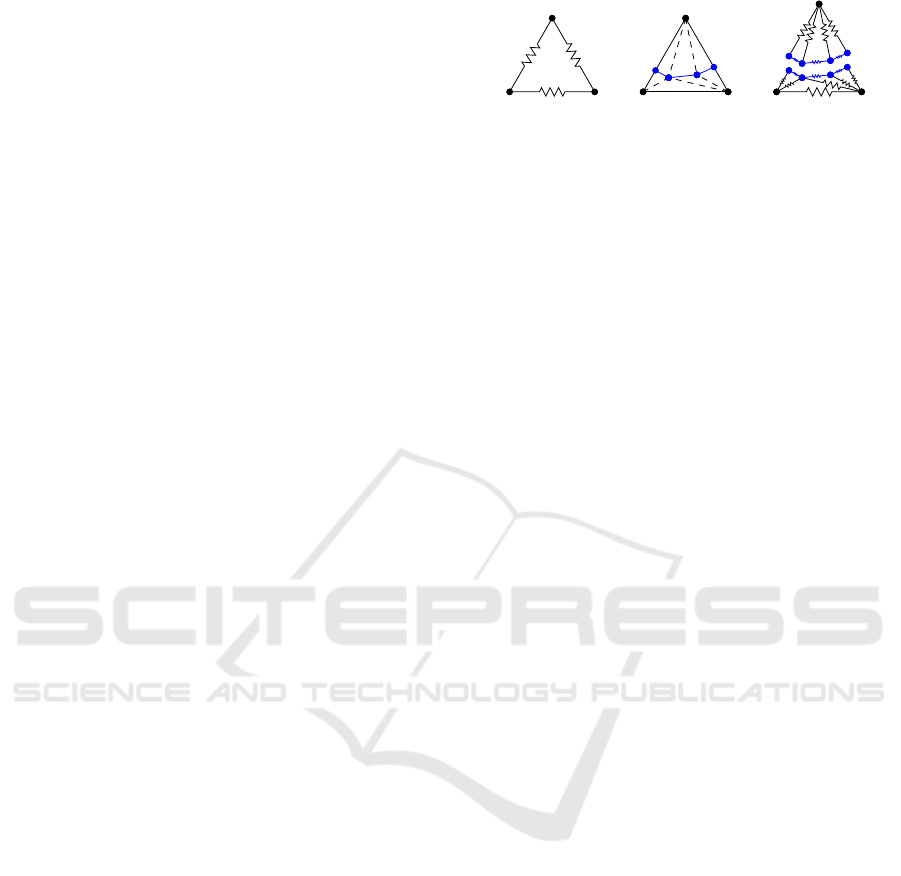
Figure 1: Cutting by element reﬁnement. Left: The un-

cut MSDM triangle. Center: Cut (blue) separates render

triangle into two polygons (triangulated). Right: MSDM

representation with increased anisotropic behavior.

The hybrid mesh approach of the “element dupli-

cation” method can fulﬁll both requirements as render

and physics mesh are decoupled, allowing a higher

render mesh resolution while physics mesh element

geometry is preserved. This method was ﬁrst intro-

duced by Molino et al. as “virtual node algorithm”

which still limited element subdivision and cut rep-

resentation (Molino et al., 2004). Sifakis et al. im-

proved on this, outlining a complex cutting algorithm

for arbitrary cuts on tetrahedral meshes with no limit

to tetrahedron subdivision (Sifakis et al., 2007). Wang

et al. present a simpler and faster algorithm for tri-

angular and tetrahedral meshes which sacriﬁces cut

accuracy, however, by using ﬂags for cut representa-

tion on a triangle (Wang et al., 2014). The cutting al-

gorithm presented in Section 4 incorporates elements

from all aforementioned hybrid mesh approaches.

The BBTT introduced in Section 5.1 relies on

the recursive partitioning of space to efﬁciently query

for all elements within a speciﬁed area. Similar to

this approach, octrees recursively partition 3D space

along three axis-aligned planes (Meagher, 1982). Bi-

nary space partitioning uses arbitrarily placed planes

which subdivide intersected objects (Schumacher,

1969; Fuchs et al., 1980). When storing points instead

of volumes, as PCDs do, k-d-trees partition space at

the median point along an axis at each node. Points

above/below that point are stored with the node’s chil-

dren, the axis used for partitioning depends on the tree

level (Bentley, 1975). Several more concepts exist,

but an exhaustive list is beyond the scope of this paper.

Compared to the structures presented here, BBTTs

can handle atomic volumes intersecting partitioning

planes, whereas PCDs, under certain conditions, can

perform merge operations in constant time.

3 ALGORITHM PREREQUISITES

This section presents the MSDM and the hybrid mesh

structure required for the cutting algorithm introduced

in Section 4.

Accurate Cutting of MSDM-Based Hybrid Surface Meshes

189

3.1 Mass-Spring-Damper Model

The MSDM is a graph-based physics simulation

model. The mass of the simulated object is distributed

among the model’s vertices. The model’s massless

edges handle the object’s internal forces, with each

edge acting as an ideal spring and an ideal damper.

An ideal spring creates a force proportional to its

axial deformation:

⃗

S(A,B)

⃗p

−⃗p

⃗p

−⃗p

· k ·



⃗p

−⃗p

− l

0(A,B)



, (1)

where

⃗

S(A,B)

is the force exerted on vertex A by a

spring anchored to vertices A and B with a spring con-

stant k and a tension-free length of l

0(A,B)

. ⃗p

and ⃗p

denote the position vectors of vertices A and B.

An ideal damper creates a force proportional to

the speed of its axial deformation:

⃗

D(A,B)

⃗p

−⃗p

⃗p

−⃗p

· c ·

(⃗v

−⃗v

) · (⃗p

−⃗p

)

⃗p

−⃗p

, (2)

where

⃗

D(A,B)

is the force exerted on vertex A by a

damper anchored to vertices A and B with a dampen-

ing coefﬁcient c. ⃗v

and⃗v

denote the velocity vectors

of vertices A and B.

The MSDM evolves by updating its vertex posi-

tions based on the accelerations induced by internal

and external forces. The force exerted on a vertex can

be calculated as follows:

⃗

E(A)

∑

B∈N(A)

⃗

S(A,B)

⃗

D(A,B)

, (3)

where

⃗

is the resulting force exerted on vertex A and

⃗

E(A)

is the sum of external forces on vertex A, e.g.

gravity or forces induced by objects in contact with

the model. N(A) is the set of vertex A’s neighbors.

The acceleration of a vertex A can be determined

using Newton’s second law of motion:

⃗

= m

·⃗a

(4)

where ⃗a

is the acceleration vector of vertex A with

mass m

. Using the forward Euler method, the veloc-

ities and positions can be updated as follows:

⃗v

A,n+1

=⃗v

A,n

+⃗a

A,n

· δt (5)

⃗p

A,n+1

= ⃗p

A,n

+⃗v

A,n

· δt (6)

3.2 Hybrid Mesh Structure

A hybrid mesh consists of the physics mesh, used for

the MSDM-based simulation, and a render mesh used

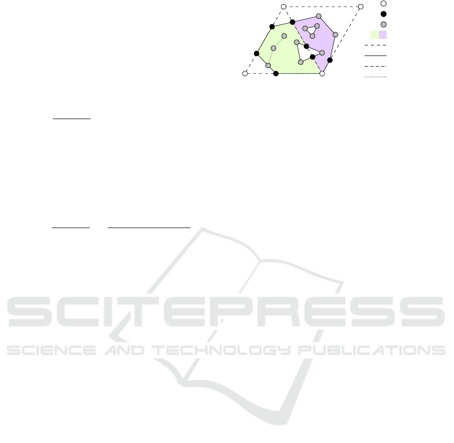
for visualization. Figure 2 illustrates the paper’s nam-

ing convention for the different node and edge types.

fgphysics node

fgboundary node

fginner node

fgrender areas

fgphysics edge

fgcontour edge

fgshared edge

fginternal edge

Figure 2: Elements of the proposed hybrid mesh.

Physics nodes and edges form the physics mesh, a

triangle mesh which is a one-to-one representation of

the MSDM-graph used for the physics simulation.

Boundary nodes lie on physics edges between

physics nodes and can be shared between physics tri-

angles. Inner nodes lie within a physics triangle. Con-

tour edges have a render area on only one edge side.

Shared edges lie on a physics edge section and con-

nect two render areas of different physics triangles.

Internal edges have the same render area on both sides

and represent discontinuities, e.g. cuts.

The render mesh is a polygon mesh where each

physics triangle contains one render polygon with

an arbitrary number of holes. Render polygons are

formed from render nodes and edges. Render nodes

can be of any type, render edges can be contour,

shared or internal. Render triangles are created by

polygon triangulation where internal edges are omit-

ted and no additional vertices are introduced.

4 CUTTING ALGORITHM

The proposed cutting algorithm works for hybrid sur-

face meshes with the aforementioned structure (see

Section 3.2) which are being cut by a triangulated cut-

ting mesh. The algorithm handles one physics triangle

at a time, ensuring neighboring physics triangles are

in a consistent state. The assumption is that the cut-

ting algorithm is applied frequently (e.g. each frame)

and that within each application only a small number

of physics triangles is cut.

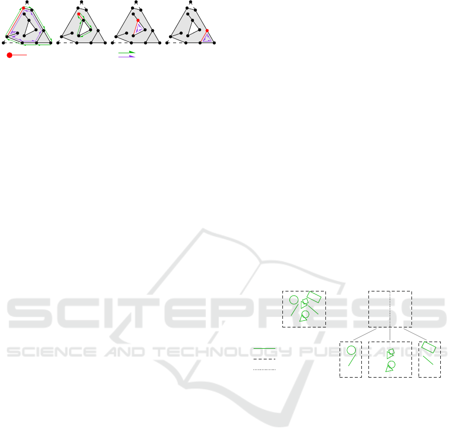
Each cut physics triangle is handled in ten steps

which are illustrated in Figure 3 and are further de-

scribed in Sections 4.1 to 4.10. Within each physics

triangle, the steps 2 to 5 should be applied for each

cutting mesh triangle individually (as opposed to ap-

plying each step once for the whole cutting mesh) be-

fore proceeding to step 6. The reasons for this ap-

proach is that in the “Cut Along Segments” step cut-

ting lines, produced by a cutting mesh triangle, are

transformed into nodes and edges. These have to be

considered by subsequently processed cutting lines in

merge/join operations.

The majority of the algorithm is performed on the

GRAPP 2023 - 18th International Conference on Computer Graphics Theory and Applications

190

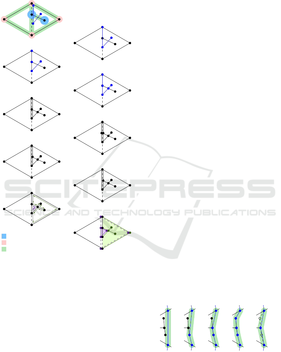
1. Detect Cutting Lines

2. Merge Cut Endpoints

3. Merge Existing Nodes

4. Join Edge Intersections

5. Cut Along Segments

6. Copy Boundary Nodes

7. Merge Adjacent Edges

8. Copy Physics Nodes

9. Detect Disjoint Polygons

10. Copy Physics Triangles

(here no effect)

fgcut merge distance δ

fgnode merge distance δ

fgedge merge distance δ

Figure 3: Steps of the proposed cutting algorithm (see Sec-

tion 4). The initial mesh consists of two physics triangles

with one congruent render triangle each.

2D tension-free physics triangle, as this simpliﬁes cal-

culations. In contrast to a node’s current position in

3D space, its position on the tension-free physics tri-

angle stays constant and can therefore be saved over

algorithm iteration boundaries.

The algorithm uses merge distances similar to

Wang et al. to compensate for ﬂoating point errors

(Wang et al., 2014), limit element size and enhance

cut continuity. As merges are performed on the

tension-free physics triangle, these distances effec-

tively change with deformations in 3D space, which

has to be considered when deﬁning them. It is as-

sumed that the deformation of objects is in most cases

limited and the impact therefore manageable.

4.1 Detect Cutting Lines

For each cutting triangle, the intersection line with

the physics triangle’s plane is calculated. These lines

are then mapped onto the tension-free physics trian-

gle (e.g. via barycentric coordinates). To compensate

for ﬂoating point errors, cutting line endpoints within

from each other are merged. Subsequent algorith-

mic steps are performed in the 2D coordinate system

of the tension-free physics triangle.

4.2 Merge Cut Endpoints

In this step, cutting line endpoints are merged to ex-

isting nodes and edges, where node merges are prior-

itized. A cutting line endpoint within merge distance

from an existing node is merged to it. Nodes which

were part of a cut in the algorithm’s previous itera-

tion are prioritized and use a larger merge distance

. Similarly, an endpoint within δ

from an existing

edge is merged onto it and subsequently checked for

node merges with the edge’s endpoints. Merge dis-

tances are illustrated in step 1 of Figure 3 and have to

be greater than the maximum ﬂoating point error δ

≥ δ

> δ

(7)

As long as Equation (7) is satisﬁed, the merge dis-

tances can be chosen freely. Note that δ

is also used

to merge nodes along cutting lines (see Figure 4).

4.3 Merge Existing Nodes

To join existing nodes and edges along cutting lines,

nodes within δ

from a cutting line are merged into it,

transforming it into a polygonal chain. As this merge

process may bring other nodes within the merge dis-

tance from the polygonal chain, this is recursively

repeated until no unmerged nodes are found within

(see steps 1 to 4 of Figure 4). In each iteration,

all nodes within δ

from a line segment have to be

merged simultaneously, as merging only one at a time

may move other nodes out of the merge distance.

1. 2. 3. 4. 5.

Figure 4: Merging nodes along a cutting line. 1.-4.: Recur-

sively merging existing nodes. 5.: Merging adjacent edges.

Accurate Cutting of MSDM-Based Hybrid Surface Meshes

191

4.4 Join Edge Intersections

Where cutting lines intersect each other or existing

edges in a non-coincident manner, intersections are

transformed into nodes and the respective lines and

edges are split into two. This results in polygonal

chains which have no intersections along their line

segments and no nodes within a distance δ

due to

the previous “Merge Existing Nodes” step.

4.5 Cut Along Segments

In this step, the cutting lines are applied to the hybrid

mesh structure. Lines outside the physics triangle’s

render area are discarded. Remaining unmerged line

endpoints are converted into nodes. Similarly, end-

points merged onto edges are converted and the re-

spective edges subdivided. Cuts along contour or in-

ternal edges have no effect, cuts along shared edges

subdivide them into two contour edges respectively.

Cutting lines non-coincident with existing edges are

converted into internal edges.

4.6 Copy Boundary Nodes

A boundary node requires duplication when the

physics triangles the node is a part of are no longer

connected by the node’s shared edges (step 6 of Fig-

ure 3 illustrates both cases). Note that boundary nodes

can be connected to up to three physics triangles (e.g.

the lower cut node in Figure 5).

4.7 Merge Adjacent Edges

Certain geometries like a straight polygonal chain

with no edges branching off needlessly complicate the

hybrid mesh structure. Therefore, nodes are omitted

if they fulﬁll all of the following criteria:

• The node is part of a cutting line.

• The node is a boundary or inner node.

• The node has only two connected edges which are

of the same kind and, in the case of shared edges,

connect the same physics triangles.

• A line connecting the node’s two neighbors has

these three nodes, but no other ones, within δ

• The node is not part of a render triangle.

Such nodes and their connected edges are replaced

by edges connecting the respective two neighboring

nodes (see step 5 of Figure 4).

4.8 Copy Physics Nodes

This step requires the node-triangle-union (NTU)

concept, which has similarities to the one-ring op-

erations by Molino et al. (Molino et al., 2004). An

NTU is seeded with a physics triangle and one of its

physics nodes. Physics triangles sharing an edge with

a physics triangle in the NTU, where the shared edge

lies on a physics edge connected to the seed node,

are recursively added. The resulting NTU is a set of

physics triangles (see Figure 5).

fgNTU seed node

fgNTU seed triangle

fgrender areas

fgNTU

Figure 5: NTUs formed after physics triangles have been

disconnected by cut.

If cuts sever all shared edges between a physics

triangle pair, the respective physics nodes may require

duplication. For each of the two physics nodes an

NTU is formed, seeded with the respective node and

one of the pair’s physics triangles. If an NTU does not

contain the physics triangle pair, the respective seed

node is duplicated. The duplicate then replaces the

seed node in all physics triangles of the NTU. In the

examples shown in Figure 5, the NTUs in the bottom

row would receive a copy of the respective seed node.

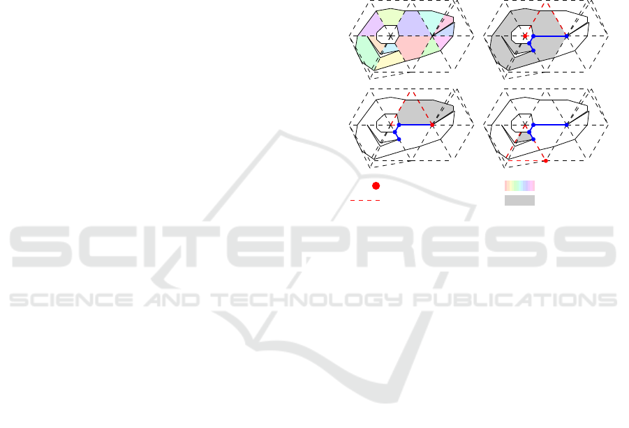
4.9 Detect Disjoint Polygons

To detect disjoint polygonal render areas a sweep

line algorithm was developed, taking inspiration from

Berg et al.’s polygon triangulation method (Berg et al.,

1997). A physics triangle’s nodes are processed pri-

marily top to bottom, secondarily left to right.

For each node, incident render edges connected to

the physics triangle are processed based on their angle

on the node’s unit circle. This angle is determined

by placing the normalized vector pointing from the

currently processed node to the edge’s other node on

a unit circle. Edges within the radian interval ]π,2π]

are processed in ascending angle order, edges outside

that interval are handled by a preceding node.

GRAPP 2023 - 18th International Conference on Computer Graphics Theory and Applications

192

fgunused

fghull

fghole fgunused fghull

fgcurrent node/edge fgleft/right polygon

Figure 6: Walks formed during the “Detect Disjoint Poly-

gons” step. Colored text marks the polygon types.

For each render edge, the counterclockwise or left

side is handled ﬁrst, the clockwise or right side sec-

ond. Each edge side is categorized as part of a poly-

gon’s “hull”, a polygon’s “hole” or “unused”.

To determine the type of a left edge side, an inﬁ-

nite line is drawn from the current node to the left. If

this line intersects an edge side, the current edge side

is a hole in the same polygon as the edge side to the

left, otherwise the current edge side is unused. A right

edge side is a hull if the side is rendered, or unused

otherwise. An edge side’s state is propagated to other

edge sides by walking along the current edge, the cur-

rent side to the left, and taking the next left on each

vertex until a closed walk is formed. The edge sides

on the left side of the walk share a state and therefore

don’t have to be handled further (see Figure 6).

4.10 Copy Physics Triangles

If more than one polygon was detected within the

physics triangle, a new physics triangle is created for

each polygon and the physics triangle’s nodes are du-

plicated for its neighbors. All affected physics tri-

angles are then joined with each other along shared

edges, such that the physics nodes of the physics edge

the shared edge lies on are merged with each other.

Once this has been done for all shared edges connect-

ing pairs of the affected physics triangles, the new

physics mesh structure is determined and changes are

propagated to the MSDM simulation.

The elements of affected physics triangles have

to be updated accordingly. Inner nodes and inter-

nal edges along the separation lines between the new

physics triangles have to be duplicated, transforming

internal edges into boundary ones. A boundary node

has to be duplicated if connected physics triangles no

longer share the same physics edge the node lies on.

Finally, the render areas of the physics triangle dupli-

cates have to be triangulated for rendering purposes,

where internal edges can be ignored. Note that trian-

gulation of the physics triangle render area in other

steps is not required, as cuts which do not subdivide

the physics triangle are not visually discernible due

to the resolution of the MSDM simulation, and nodes

that are part of a render triangle are exempted from

the “Join Edge Intersections” step.

5 AUXILIARY DATA

STRUCTURES

This section presents two data structures developed

for use with the proposed cutting algorithm. Both

data structures are optional, but can improve its ef-

ﬁciency in scenarios where physics triangles contain

large node and edge numbers. The BBTT is an al-

ternative to octrees and is used to query for objects

whose BB intersects a given BB. The PCD allows

to efﬁciently query for all points within a predeﬁned

merge distance. Both data structures may prove use-

ful in other application areas as well.

5.1 Bounding Box Ternary Tree

A bounding box ternary tree (BBTT) is a space parti-

tioning data structure where each node encompasses

a volume deﬁned by its BB and stores elements fully

contained within. A parent node has a split plane in-

tersecting its BB center orthogonal to the axis with the

longest BB extent. It stores elements below/above/in-

tersecting this plane in its lower/higher/centric child

node. A leaf node stores elements in a collection.

⇒

fgelement

fgnode’s BB

fgsplit plane

Figure 7: Split of a BBTT node as its capacity is exceeded.

When a leaf node’s element count exceeds a soft

limit it tries to distribute its elements among three new

child nodes (see Figure 7). Child nodes created by

such a node split inherit the parent’s BB. The lower/

higher child has its BB maximum/minimum value

along the split axis trimmed to the split plane. The

centric child and future children thereof lose the abil-

ity to split along the respective split axis. At root node

level all axes are divisible; if a leaf node has no re-

maining divisible axis it cannot be split further.

5.2 Point Cluster Dictionary

A point cluster dictionary (PCD) is used where points

are clustered together within a merge distance δ

. It

divides each axis into indexed segments of width

w = δ

+ δ

(8)

where δ

> δ

, forming square/cubical elements in

2D/3D, and uses 3/4 nested dictionaries to store clus-

Accurate Cutting of MSDM-Based Hybrid Surface Meshes

193

ter centers. Segment indices are used to access an el-

ement’s dictionary which stores cluster centers based

on their position.

For an arbitrary point, all stored cluster centers

within δ

can be found in the point’s encompassing

element or adjacent elements. When limiting stored

cluster centers, such that no two are within δ

of each

other, the number of cluster centers per element is

limited as well, allowing to ﬁnd all stored cluster cen-

ters within δ

to an arbitrary point in time O(1).

6 RESULTS

Tests were carried out on a hybrid mesh consisting of

12 equilateral physics triangles with an initially con-

gruent render mesh, simulated by a single-threaded

MSDM simulator performing around 63,000 updates

per second. δ

/δ

were set to approximately

4000

of the equilateral triangle side length. It

is assumed that for most applications a signiﬁcantly

higher number of elements would be used, but the

manageable amount here sufﬁces to illustrate the cut-

ting algorithm and simpliﬁes analysis.

Cutting tests were performed using either man-

ually triggered cutting meshes consisting of one or

more triangles, or automatically applied meshes cre-

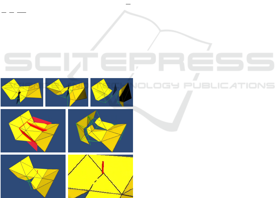
ated each frame by a moving cutting edge. A few se-

Figure 8: Cutting of hybrid mesh with initially congruent

physics (green) and render mesh (yellow), anchored along

two sides. Top

: Incremental cutting using a single triangle.

Center

: E-shaped cutting mesh consisting of ten triangles.

Bottom

: Discontinuity while cutting with moving edge.

video: https://youtu.be/5j6pCwGJkL0

video: https://youtu.be/uAPdq4VuTyY

video: https://youtu.be/Lq37PHJRUsI

lected examples are illustrated in Figure 8. Cuts along

existing nodes and edges separate the mesh without

creating new MSDM elements, cuts through render

areas are registered but do not lead to subdivision un-

til disjoint polygons are formed. The cutting algo-

rithm therefore performs as expected in most parts,

although some shortcomings have been identiﬁed:

• Discontinuous Cutting Lines

Discontinuities can arise when both cutting line

endpoints are merged to the same position even

though a second, better suitable but lower priority

merge option exists, or when a physics simulation

update moves a node that was previously merged

to out of merge distance of the cutting mesh.

• Incomplete Physics Mesh Handling

Properties outside the hybrid mesh structure pre-

sented in Section 3.2 are not considered by the al-

gorithm, e.g. whether a node is anchored in space

(see center right image of Figure 8).

• Physics Triangles Freely Rotate Around Edges

The hybrid mesh model does not include MSDM

edges for bending resistance.

These issues will have to be addressed in future work

(see solution approaches in Section 7).

7 CONCLUSIONS AND FUTURE

WORK

The cutting algorithm presented in this paper success-

fully uses the hybrid mesh approach (partial separa-

tion of physics simulation and render mesh) to com-

bine accurate cut representation on the render mesh

with preservation of the original MSDM element ge-

ometry for surface meshes, although some additional

mass is introduced as physics nodes are copied. The

load for the MSDM simulation increases as physics

triangles are duplicated (similar to other hybrid mesh

cutting methods) but introduces far fewer elements

than cutting by element reﬁnement (see Figure 1),

which provides comparable cut accuracy. Introduc-

tion of new elements on the render mesh is also

limited by merge distances, which balance element

creation with cut accuracy. The cutting algorithm’s

major downside is its high algorithmic complexity.

Projecting cuts on the tension-free 2D geometry of

physics triangles reduces the complexity of individ-

ual calculations though and allows to store positional

data over iteration boundaries.

The presented BBTT, similar to octrees and bi-

nary space partitioning, recursively subdivides space

but does not require a collision-free separation plane

GRAPP 2023 - 18th International Conference on Computer Graphics Theory and Applications

194

to do so. Its structure also allows further subdivi-

sion of nodes holding plane-intersected elements to

the point where a node represents a single point in

space and stores only elements whose minimum BB

intersects that point. This should make it a viable

alternative to octrees and binary space partitioning,

especially in scenarios where placement of collision-

free separation planes is challenging. The presented

point clustering method is more specialized but excels

when points are clustered within a predeﬁned δ

The cutting algorithm and its auxiliary data struc-

tures would however beneﬁt from additional valida-

tion and performance tests. Testing the algorithm on

a wider range of meshes and direct comparison with

existing hybrid mesh cutting algorithms would be de-

sirable as well. Future work will also have to address

the shortcomings found during testing (listed in Sec-

tion 6). For these, the following solution approaches

are proposed:

• Discontinuous Cutting Lines

Where both cutting line endpoints would be

merged to the same position, the two best dis-

tinct merge options should be used instead. Ad-

ditionally, a point P merged to a node N should

be used as an additional cluster center for N in the

subsequent algorithm iteration in cases where P is

within merge distance of N’s original position.

• Incomplete Physics Mesh Handling

A physics node’s anchor property should only be

copied if it is part of a render polygon.

• Physics Triangles Freely Rotate Around Edges

Wherever a physics triangle pair shares a physics

edge, an additional MSDM edge should be placed

between the two unshared physics nodes. These

would have to be considered when a physics tri-

angle’s neighborhood changes.

A fully parallelizable version of the algorithm

may be necessary for cases where a large number of

physics triangles are cut at once as well. Finally, a

strategy to effectively expand merge distances over

physics triangle boundaries should be incorporated.

Work on these issues is expected to be continued at

some point, although no time table can be given here.

ACKNOWLEDGEMENTS

This project is ﬁnanced by research subsidies granted

by the government of Upper Austria within the re-

search projects MIMAS.ai and MEDUSA (FFG grant

no. 872604). RISC Software GmbH is Member of

UAR (Upper Austrian Research) Innovation Network.

REFERENCES

Bentley, J. L. (1975). Multidimensional binary search trees

used for associative searching. Communications of the

ACM, 18(9):509–517.

Berg, M. d., Kreveld, M. v., Overmars, M., and

Schwarzkopf, O. C. (1997). Polygon triangulation. In

Computational geometry, pages 45–61. Springer.

Bielser, D., Maiwald, V. A., and Gross, M. H. (1999). In-

teractive cuts through 3-dimensional soft tissue. In

Computer Graphics Forum, volume 18, pages 31–38.

Wiley Online Library.

Cotin, S., Delingette, H., and Ayache, N. (2000). A hy-

brid elastic model allowing real-time cutting, defor-

mations and force-feedback for surgery training and

simulation. Visual Computer, 16(8):437–452.

Fuchs, H., Kedem, Z. M., and Naylor, B. F. (1980). On

visible surface generation by a priori tree structures.

In Proceedings of the 7th annual conference on Com-

puter graphics and interactive techniques, pages 124–

133.

Meagher, D. (1982). Geometric modeling using octree en-

coding. Computer graphics and image processing,

19(2):129–147.

Molino, N., Bao, Z., and Fedkiw, R. (2004). A virtual

node algorithm for changing mesh topology during

simulation. ACM Transactions on Graphics (TOG),

23(3):385–392.

Nienhuys, H.-W. and van der Stappen, A. F. (2000). Com-

bining ﬁnite element deformation with cutting for

surgery simulations. In EUROGRAPHICS (short pre-

sentations).

Schumacher, R. (1969). Study for applying computer-

generated images to visual simulation, volume 69. Air

Force Human Resources Laboratory, Air Force Sys-

tems Command.

Sifakis, E., Der, K. G., and Fedkiw, R. (2007). Arbitrary

cutting of deformable tetrahedralized objects. In Pro-

ceedings of the 2007 ACM SIGGRAPH/Eurographics

symposium on Computer animation, pages 73–80.

Steinemann, D., Harders, M., Gross, M., and Szekely, G.

(2006). Hybrid cutting of deformable solids. In IEEE

Virtual Reality Conference (VR 2006), pages 35–42.

IEEE.

Wang, M. and Ma, Y. (2018). A review of virtual cutting

methods and technology in deformable objects. The

International Journal of Medical Robotics and Com-

puter Assisted Surgery, 14(5):e1923.

Wang, Y., Jiang, C., Schroeder, C., and Teran, J. (2014).

An adaptive virtual node algorithm with robust mesh

cutting. In Symposium on Computer Animation, pages

77–85.

Wu, J., Westermann, R., and Dick, C. (2015). A survey

of physically based simulation of cuts in deformable

bodies. In Computer Graphics Forum, volume 34,

pages 161–187. Wiley Online Library.

Accurate Cutting of MSDM-Based Hybrid Surface Meshes

195