Depression in Obstructive Sleep Apnea Patients: Is Using Complex Deep

Learning Structures Worth It?

Mostafa Moussa

, Yahya Alzaabi and Ahsan Khandoker

Department of Biomedical Engineering, Khalifa University of Science and Technology, Abu Dhabi, 127788, U.A.E.

Keywords:

Depression, Electroencephalography, Electrocardiography, Breathing Signals, Gated Recurrent Unit Long

Short-Term Memory Networks.

Abstract:

The prevalence and severity of depression make it imperative to develop a means to automatically detect it, so

as to alleviate the associated mental effort and cost of seeing a dedicated professional. Depression can also

co-exist with other conditions, such as Obstructive Sleep Apnea Syndrome (OSAS). In this paper, we build

upon our previous work involving sleep staging, detection of OSAS, and detection of depression in OSAS

patients, but focus solely on the latter of the three. We use features extracted from EEG, ECG, and breathing

signals of 80 subjects suffering from OSAS and half of which also with depression, using 75 % of this 80-

subject dataset for training and 10-fold cross-validation and the remainder for testing. We train three models

to classify depression: a random forest (RF), a three-layer artiﬁcial neural network (3-ANN), and a gated-

recurrent unit long short-term memory (GRU-LSTM) recurrent neural network. Our analysis shows that, like

our previous work, the 3-ANN is still the best performing model, with the GRU-LSTM following closely

behind at an accuracy of 79.0 % and 78.6 %, respectively, but with a smaller F1-score at 80.0 % and 81.6 %.

However, we believe that the large increase in computation time and number of learnable parameters does not

justify the use of GRU-LSTM over a simple ANN.

1 INTRODUCTION

Major Depressive Disorder (MDD) is a common men-

tal disorder characterized by reduced production of

certain neurotransmitters in the brain that affects 10

% of the population (Gao et al., 2018). Patterns de-

scribed by Murray et al. in (Murray et al., 2012) show

that depression is consistently on the rise as a preva-

lent cause of morbidity or disability and its effects in-

clude but are not limited to, memory loss, irritabil-

ity, loss of interest, disordered sleep (insomnia or hy-

persomnia) and eating (weight loss or gain), tiredness

and lethargy, anxiety, reduced cognitive and/or mo-

tor performance, feelings of inadequacy, inability to

concentrate, self-harm or suicidal ideation or attempt,

and unexplained physical pain (Strock, 2002).

Obstructive Sleep Apnea Syndrome (OSAS) is a

condition characterized by cessation of breathing dur-

ing sleep speciﬁcally due to airway blockages pri-

marily caused by muscles, mainly the genioglossus.

Though OSAS is not as prevalent as depression and

has vastly differing causes, it can still occur in pa-

https://orcid.org/0000-0003-4977-355X

tients with depression, or vice versa. It is thus not un-

likely that a selected dataset of OSAS patients would

include those with depression as well, as is the case

in our previous works and this current one (Moussa

et al., 2022). Though depression was an important

part of these previous works, OSAS was the main fo-

cus and depression was classiﬁed as a comorbidity.

From the literature, we know sleep apnea and hy-

popnea are correlated with lower quality of life in

general including in large part psychological health.

That is to say depression is relatively prevalent in

people who suffer from OSAS (Yue et al., 2003;

ornsd

ottir et al., 2016; Ejaz et al., 2011). In one

of the aforementioned works, Yue et al. found that

the 30 patients suffering from sleep apnea and hypop-

nea have higher scores for depression with a t-value

of 2.62 (P ¡ 0.05) (Yue et al., 2003).

In the literature, we have seen plenty of works

wherein the authors use electrophysiological signals,

such as ECG (Zang et al., 2022) or EEG (Mumtaz

et al., 2018; Hosseinifard et al., 2013) in classify-

ing major depressive disorder or depression. The

use of varying machine learning algorithms played

a critical role in classiﬁcation in these works, which

Moussa, M., Alzaabi, Y. and Khandoker, A.

Depression in Obstructive Sleep Apnea Patients: Is Using Complex Deep Learning Structures Worth It?.

DOI: 10.5220/0011655600003414

In Proceedings of the 16th International Joint Conference on Biomedical Engineering Systems and Technologies (BIOSTEC 2023) - Volume 4: BIOSIGNALS, pages 203-211

ISBN: 978-989-758-631-6; ISSN: 2184-4305

 2023 by SCITEPRESS – Science and Technology Publications, Lda. Under CC license (CC BY-NC-ND 4.0)

203

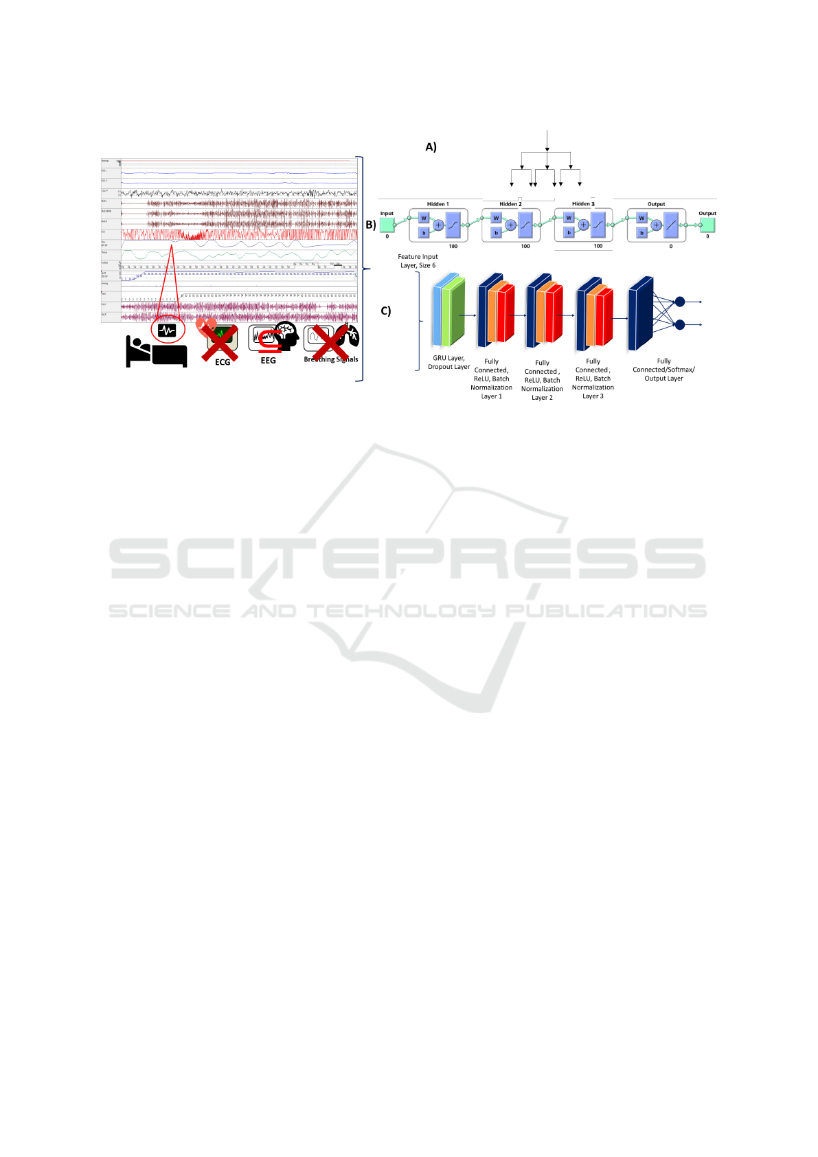
Figure 1: Summary of data extraction and feature selection, and representations of the A) random forest, B) 3-ANN, and C)

GRU-LSTM. The red crosses and subset symbol over the signal labels represent feature selection - no features selected from

ECG and breathing signals, and only 6 features selected from the EEG.

further supports our solution. Zang et al. use raw

ECG recordings of 74 subjects as input to their CNN

and obtain an accuracy of 93.96 %, a sensitivity of

89.43 %, a speciﬁcity of 98.49 %, and an F1-score

of 93.67 % (Zang et al., 2022). Mumtaz et al. use

support vector machines (SVM), logistic regression

(LR), and Naive Bayes (NB) with EEG synchroniza-

tion likelihood (SL) features from 64 subjects. They

obtained the best results at an accuracy of 98.00 %,

a sensitivity of 99.9. %, a speciﬁcity of 95.00 %

and an F1-score of 97.00 % with SVM with 10-fold

cross-validation (Mumtaz et al., 2018). Hosseinifard

et al. use K

Nearest Neighbor (KNN), linear dis-

criminant analysis (LDA), and LR with features like

average band powers, detrended ﬂuctuation analysis

(DFA), Higuchi fractal dimension, correlation dimen-

sion and Lyapunov exponent extracted from the EEG

data of 90 subjects to diagnose MDD. Logistic Re-

gression yielded the best performance at an accuracy

of 90.00 %. They had used 2/3 of their set for train-

ing and leave-one-out cross-validation(Hosseinifard

et al., 2013).

A common thread among these discussed works

aside from the use of electrophysiological signals is

their goal; the authors aim to diagnose depression.

Our goal, and thus contribution, differs slightly, since

we focus only on depression in subjects we know

suffer from OSAS forming a novel dataset (Moussa

et al., 2022).

Figure 1 gives an abstract idea of our methodol-

ogy, as well as the architectures/algorithms we used

in our work. The contribution in our work lies

mainly in classiﬁcation of depression in OSAS with

the novel dataset via machine learning and a simple

deep learning architecture, and gauging what would

make switching to deep learning worth the increase in

computational cost and subsequently, physical cost.

2 METHODOLOGY

2.1 Dataset and Processing

Seeing the extensive use of electrophysiological sig-

nals for classiﬁcation of depression, we elected to use

electroencephalography (EEG), electrocardiography

(ECG), and breathing signals for that purpose. We fo-

cus particularly on depression in subjects that are suf-

fering from OSAS, so while our results may not nec-

essarily be applicable to the general population, they

can provide a suitable baseline for OSAS patients. For

the purpose of detecting depression alone in OSAS

patients, we use a subset of the dataset described in

our previous work (Moussa et al., 2022); instead of

using the electrophysiological signals of 118 subjects,

we use that of 80 subjects. These 80 subjects consist

of 40 with depression and OSAS and 40 with OSAS

alone, collected from the American Center of Psy-

chiatry and Neurology (ACPN) in Abu Dhabi, UAE,

meaning we omit the 6 healthy subjects from this set

and the 32 supplementary healthy subjects from the

STAGES dataset (Zhang et al., 2018). The 80 sub-

jects selected only from the original study, excluding

the STAGES healthy subjects, consist of 48 male sub-

jects and 32 female, all UAE Nationals between the

ages of 20 and 66 with a mean age of 44.2 ± 10.9

BIOSIGNALS 2023 - 16th International Conference on Bio-inspired Systems and Signal Processing

204

years-old at the time of the study. This study was ap-

proved by the Institutional Review Board (IRB) of the

ACPN on the 2

of October, 2017 with IRB reference

number 0019.

Among the 80 subjects, 2 had an Apnea-

Hypopnea Index (AHI) less than 5, 27 had an AHI

between 5 and 15, 27 had an AHI between 15 and

30, and 24 had an AHI above 30. Since we know

the status of both depression and apnea, we can train

supervised machine learning models to classify our

subjects into one of two classes: depressed or not de-

pressed, both with OSAS. We can also better partition

them according to AHI, sleep stage, and depression

status to further investigate the effects of certain con-

ditions on classiﬁcation performance in other works,

as we did for sleep stages in (Moussa et al., 2022).

As previously stated, we primarily use EEG, ECG,

and breathing signals, namely airﬂow, oxygen satura-

tion, and thoracic effort, in addition to other informa-

tion ”signals”, such as the hypnogram detailing sleep

stages. These are not the only recorded signals, how-

ever. The subjects undergo overnight polysomnog-

raphy, which conventionally include the aforemen-

tioned signals in addition to chin and leg electromyo-

graphy (EMG), electrooculography (EOG) for both

eyes, and abdominal effort. Chin EMG (Al-Angari,

2008; Moradhasel et al., 2021) could pave the way for

better detection of OSAS due to the more direct causal

effect between the condition and dilator muscles, and

could even facilitate the use of sensors directly with

the genioglossus muscle instead of chin placement.

The main ﬁve signals are recorded by means of

an 8-channel EEG cap for brain signals, an ECG for

heart signals, a spirometer for airﬂow, a pulse oxime-

ter for oxygen saturation, and a piezoelectric belt for

thoracic movement. The EEG channels used are O1,

O2, C3, C4, F3, and F4 with A1 and A2 according to

the 10-20 convention, as shown in Figure 2, and the

other signals are recorded via standard leads/sensors

and standard lead/sensor placement.

After obtaining the signals, some processing

would be required to ensure the data is clean and

ready for feature extraction, selection, and eventually,

classiﬁcation. Since the EEG, ECG, and breathing

signals are sampled at 200 Hz, 100 Hz, and 10 Hz,

respectively. The EEG and ECG are also put through

a 50 Hz Notch ﬁlter to remove the power-line inter-

ference and all three signals are put through band-

pass ﬁlters in previous work to be published by Yahya

Alzaabi; the breathing signals and ECG at 0.1-0.4 Hz

and the EEG at 0.5-30 Hz to keep beta, theta, alpha,

and delta waves. Following ﬁltering, the signals are

split into 5-minute intervals selected manually by in-

spection mainly based on whether or not an apnea has

Figure 2: EEG electrode conﬁguration in which the green

electrodes are those used.

occurred, so as to avoid artifacts. This results in a

total of 1,424 intervals or observations from the 118

subjects, of which 1,005 observations are from our 80

subjects. For each of these observations, we compute

a set of 34 features, 24 from EEG signals, 6 from the

ECG signals/heart rate variability (HRV), 1 directly

from airﬂow, and 3 from the interaction between air-

ﬂow and ECG/HRV, or more speciﬁcally R-R interval

(RRI) signals. The EEG features are simply average

powers extracted for each brain wave from each elec-

trode, with the exception of the reference electrodes,

the ECG features include the average very low fre-

quency, low frequency, and high frequency powers, a

normalized set of the latter two, and the ratio/division

between the latter two. The singular breathing sig-

nal/airﬂow feature is the respiratory frequency, and

the remaining three features are the respiratory sinus

arrhythmia (RSA), the normalized RSA, and the time-

dependent phase coherence between RSA and airﬂow

(phases extracted via Hilbert transform), also known

as lambda (λ).

After taking care of noise with ﬁltering and man-

ual selection of intervals and extracting our feature

set, we ﬁll in missing values using shape-preserving

piecewise cubic spline interpolation (Fritsch and Carl-

son, 1980; Kahaner et al., 1989), also known as

Pchip, then follow that by Softmax normalization,

Box-Cox transform (Box and Cox, 1964) to ensure

normal probability distribution, and z-score normal-

ization (Moussa et al., 2022). These processing steps

are described in Equations 1-3, where Data1 is the

Softmax normalized data, Data2 is Data1 with prob-

ability distribution made approximately normal, and

DataFinal is centered and standardized Data2. Box-

Cox transform is a non-linear power transform that

makes the data probability distribution approximately

normal by ﬁnding an optimal value of an exponent (λ)

Depression in Obstructive Sleep Apnea Patients: Is Using Complex Deep Learning Structures Worth It?

205

that results in the best normal distribution approxima-

tion. Looking at Equation 2, we can conclude that

Box-Cox transformation would require the input data

to be positive, which we achieve via Softmax normal-

ization before applying the power transform.

Data1 =

1 + exp

mean(Data)−Data

std(Data)

(1)

Data2(λ) =

(

Data1

−1

, i f λ ̸= 0

log(Data1), i f λ = 0

(2)

DataFinal =

Data2 − mean(Data2)

std(Data2)

(3)

Despite extracting 34 features for each observa-

tion, we do not use the full feature set in this work.

As we have seen in (Moussa et al., 2022), using

Chi

to select features whose importance score is

greater than or equal to the average feature impor-

tance score, along with the bi-layer artiﬁcial neu-

ral network (ANN) yielded the best classiﬁcation re-

sult for depression compared to other feature selec-

tion algorithms including sequential feature selec-

tion, neighborhood and principal component analysis,

maximum relevance minimum redundancy and Reli-

efF algorithms, so we opt to directly apply Chi

feature selection, ending up with six features out of

the thirty four. The six selected features by this tech-

nique are all extracted from EEG signals, also surpris-

ingly from only two channels. These features include

the average powers of beta, theta, and alpha waves

from channels F3 and F4. In the context of feature se-

lection on MATLAB, the function examines whether

each of our 34 features is independent of the depres-

sion status using individual Chi

tests. The score out-

put from this function is the negative of the common

logarithm of the p-value, and we know a small p-value

indicates that the corresponding feature is dependent

on the label is an important feature. This score would

approach inﬁnity as the p-value approaches zero. Our

analysis concluded that the aforementioned six fea-

tures have an inﬁnite score, hence were selected as

our features.

Now that signal processing has concluded, we

have a clean dataset of 1,005 observations each with

six features with an approximately normal probability

distribution and no missing values. The 80 subjects

are then split into two sets, one for training and 10-

fold cross-validation and comprises the observations

of 75 % of the subjects, and the other set for testing

and comprises the observations of the remaining 25 %

of the subjects. The labels are likewise partitioned in

the same manner, culminating in a partitioned dataset

ready to be input to machine learning algorithms.

2.2 Classiﬁers and Performance

Evaluation

As we saw in Section 1, machine learning is com-

monly used in detecting depression in the literature,

due to its automated nature, the simplicity of its met-

rics, and the insights it could help us derive regard-

ing the nature of the condition, the widely established

methods of diagnosing depression, or the features

used in classiﬁcation. In addition, it has social ben-

eﬁts as it reduces the need for human interaction in

diagnosis.

Artiﬁcial neural networks (ANNs) and deep learn-

ing techniques use the back-propagation algorithm to

minimize a loss function, and to automatically extract

features with the major difference being an added

function or layer. In convolutional neural networks,

the added function would be convolutional layers,

which, as their name suggests, convolve the input to

reduce its size, producing a smaller feature map. In

gated recurrent unit long short-term memory (GRU-

LSTM or GRU) networks, the added function(s) are

an update and reset gates that control the ﬂow of in-

formation (Erdenebayar et al., 2019).

As we have previously tested out numerous classi-

ﬁers in (Moussa et al., 2022), we opt to directly com-

pare the best-performing model in that work (ANN),

with a deep learning technique- a GRU-LSTM net-

work, and getting the results with random forest as

some form of baseline. This is because random

forests are known for their generally robust perfor-

mance and relative simplicity compared to deep learn-

ing techniques. The random forest (RF) used was the

same as the previous work; bagged trees with sur-

rogate decision split and 200 learning cycles. How-

ever, some changes were made to the ANN model

to better optimize it for the problem. The model,

named 3-ANN, now consists of three hidden layers

instead of two with 100 units each and a regulariza-

tion term (lambda) of 0.01 instead of 0 in between

the input and output layers. The GRU-LSTM model

is new, as it would have been difﬁcult to employ

prior to hardware upgrade from a machine with the

Nvidia GTX 1050Ti GPU to one with RTX 3080,

and consists of a total of 15 layers, as shown in Fig-

ures 1 and 3. These layers begin with a feature in-

put layer of size 6 × Number of training samples,

followed by a gated recurrent unit of size 10 and a

40 % dropout layer. Afterwards, we have three fully

connected layers with 50 units with batch normaliza-

tion and reLu following each one. Then ﬁnally, we

have our ”output” layer, which consists of a fully con-

nected layer with 2 units, a SoftMax layer, and the

actual output layer, since our entire analysis and net-

BIOSIGNALS 2023 - 16th International Conference on Bio-inspired Systems and Signal Processing

206

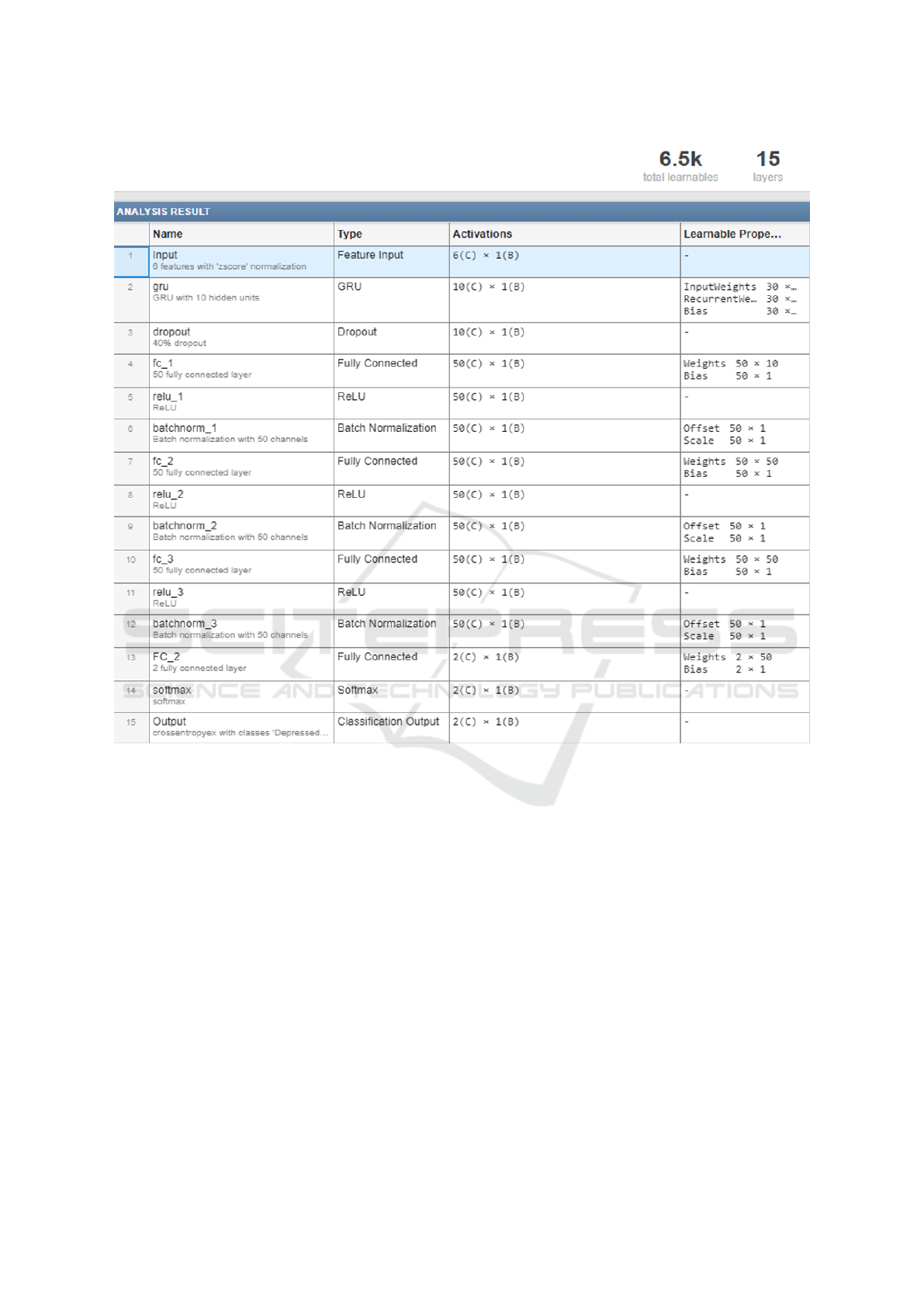
Figure 3: Layer descriptions and number of learnable parameters of the GRU-LSTM model. Each layer has the number of

units under its name and/or any additional options (i.e. normalization, dropout, number of channels).

work design are done on MATLAB. The weights are

initialized via the Glorot initializer (Glorot and Ben-

gio, 2010). The 3-ANN uses the Limited-memory

Broyden–Fletcher–Goldfarb–Shanno (LBFGS) algo-

rithm in training while the GRU uses stochastic gra-

dient descent with a momentum of 0.8. The addi-

tional training options for the GRU include a mini-

batch size of 32, a ﬁxed learn rate of 0.01, an L2-

regularization term of 0.005, a validation frequency

of 1 (each epoch), and a maximum number of epochs

of 1000. Figure 3 shows a brief description of each

layer and gives an idea about the number of associ-

ated computations.

We use 10-fold cross-validation, as stated earlier,

to ensure our models do not overﬁt. With the deep

learning model on MATLAB, this is implemented by

training a model using 9 folds and the last fold for val-

idation, and repeating while changing the validation

fold until all folds have been used for validation, and

then the model with the best validation performance

is taken. With the other two models, the implemen-

tation on MATLAB is more automatic than having to

select a model based on validation performance algo-

rithmically.

After the models are trained and validated, we

measure their performance with the testing set. Clas-

siﬁcation performance is measured by accuracy, sen-

sitivity, speciﬁcity, precision, F1-score, the area un-

der receiver operating characteristics (ROC) curve

(AUC), Cohen’s κ coefﬁcient (Cohen, 1960), and

Matthews correlation coefﬁcient (Matthews, 1975).

Accuracy measures how many instances were cor-

rectly classiﬁed, sensitivity measures the number of

instances correctly classiﬁed positive out of the actual

positive instances, speciﬁcity measures the number of

instances correctly classiﬁed negative out of the ac-

Depression in Obstructive Sleep Apnea Patients: Is Using Complex Deep Learning Structures Worth It?

207

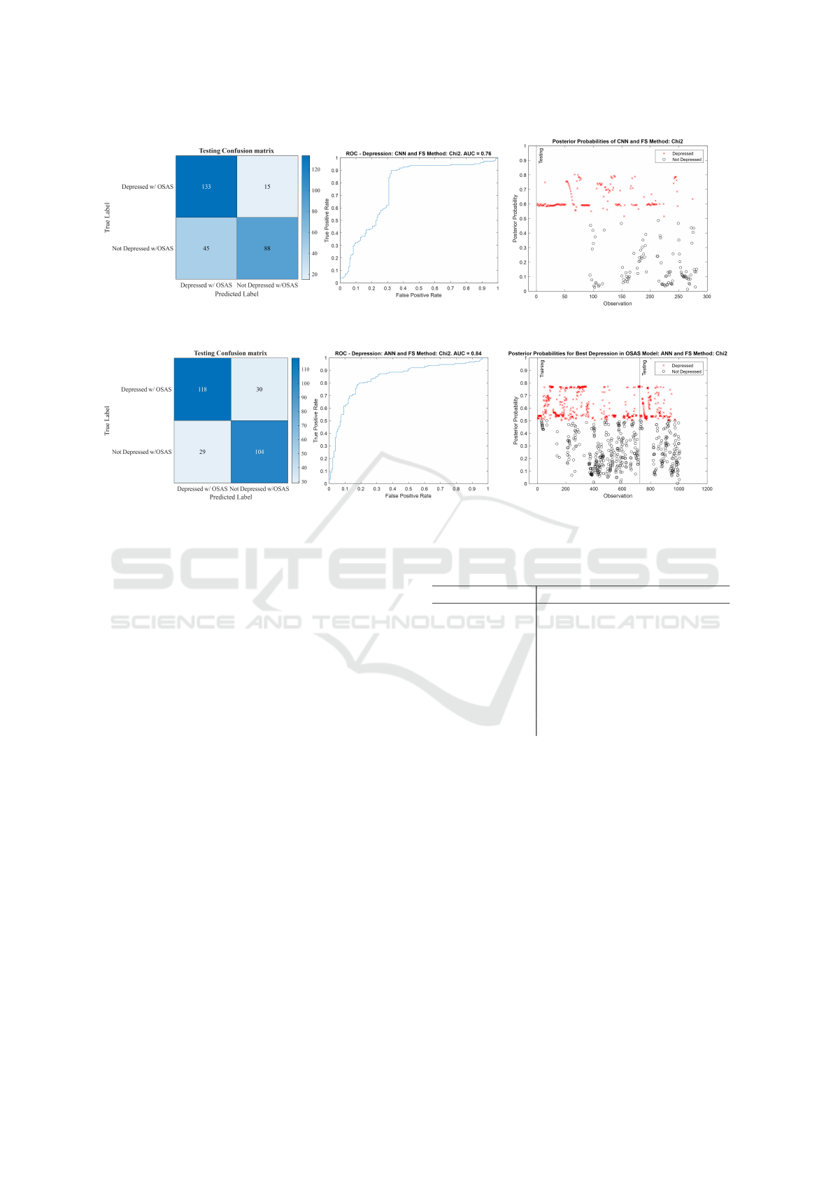
Figure 4: Testing confusion matrix, receiver operating characteristics (ROC) curve, and posterior probability plot of the 3-

ANN model.

Figure 5: Testing confusion matrix, receiver operating characteristics (ROC) curve, and posterior probability plot of the GRU

model.

tual negative instances, precision measures the num-

ber of correctly classiﬁed positive instances out of the

total number of classiﬁed positive instances, and F1-

score is a harmonic mean deﬁned as twice the prod-

uct of sensitivity and precision divided by their sum.

The AUC is a measure of class separability or essen-

tially how useful the model is at distinguishing the

classes, whereas Cohen’s κ coefﬁcient is a measure of

how much the model’s accuracy is better than chance

based on class distribution, and Matthews correlation

coefﬁcient is a correlation coefﬁcient similar to the

F1-score, and is generally known as the most infor-

mative measure of the quality of a binary classiﬁer.

3 RESULTS AND DISCUSSION

As stated earlier, we compute the testing accuracy,

sensitivity, speciﬁcity, precision, F1-score, AUC, Co-

hen’s κ coefﬁcient, and Matthews correlation coefﬁ-

cient (MCC) for the three classiﬁers. Although we

compute all metrics, we mainly look at the accuracy,

F1-score, κ, and MCC in comparison in order to make

a conclusion regarding the best classiﬁer for detecting

depression in OSAS patients with our dataset and pro-

cessing steps.

Figure 4 and Figure 5 show the testing confusion

matrix, ROC, and posterior probability plots of both

Table 1: Testing performance of the three classiﬁers in clas-

siﬁcation of depression in OSAS patients.

Model RF 3-ANN GRU-LSTM

AUC 0.71 0.84 0.76

Accuracy (%) 67.6 79.0 78.6

Sensitivity (%) 56.8 79.7 89.9

Speciﬁcity (%) 79.7 78.2 66.2

Precision (%) 75.7 80.3 74.7

F1-Score (%) 64.9 80.0 81.6

κ 0.36 0.58 0.57

MCC 0.37 0.58 0.58

of these models to better visualize the difference in

performance. Table 1 shows comparable performance

between the 3-ANN and the GRU-LSTM and shows

both beating the random forest model in all metrics

but speciﬁcity. The 3-ANN has a higher AUC, accu-

racy, speciﬁcity, precision, and κ than the GRU, but

the GRU has a higher sensitivity, F1-score and they

both have almost the same value of the Matthews cor-

relation coefﬁcient.

The reasons the performance of the two neural

network models is similar could include the relatively

small size of the available dataset, the use of only

6 out of the 34 features, the simplicity of the se-

lected features, or the simplicity of the supposedly

more complex model (GRU). The ﬁrst reason is sim-

ple enough; artiﬁcial neural networks generally re-

BIOSIGNALS 2023 - 16th International Conference on Bio-inspired Systems and Signal Processing

208

Table 2: Comparison between our model and works focused on detecting depression. OSAS: Obstructive Sleep Apnea Syn-

drome, EEG: Electroencephalography, ECG: Electrocardiography, ANN: Artiﬁcial Neural Networks, NB: Naive Bayes, LR:

Logistic Regression, KNN: K-th Nearest Neighbor, SVM: Support Vector Machine, RF: Random Forest, CNN: Convolutional

Neural Network, GRU-LSTM: Gated Recurrent Unit Long Short-Term Memory Network, LDA: Linear Discriminant Analysis.

Work (Zang et al., 2022) (Mumtaz et al., 2018) (Hosseinifard et al., 2013) Proposed Method

Main Objective Classify Depression Classify Depression

Classify MDD

Classify Depression in

OSAS patients

Dataset

74 subjects’

raw ECGs

64 subjects’

EEGs

90 subjects’

EEGs + 4 non-linear

features

1,005 observations extracted

from EEG, ECG, and

breathing signals of 80 subjects

Machine

Learning

Algorithms

CNN

LR, SVM,

and NB

KNN,

LDA,

and LR

Random Forest, 3- ANN,

GRU-LSTM

Signiﬁcance

Simplicity of

methodology: The authors

use raw ECG signals

with CNNs in their analysis

Thorough analysis for

some classic machine

learning algorithms and

features used are promising

The authors present a thorough

description of a robust methodology

to classify depression in general,

describing in detail their features,

machine learning models and cross-

validation schemes, as well as their

novel dataset

Compares best

depression in OSAS classiﬁcation

method in (Moussa et al., 2022) with deep learning

Limitations

Using CNNs with raw signals

is inconvenient in

resource-restricted environments

No signiﬁcant limitations found,

though we would be interested to see

how this setup performs with other datasets

Only the accuracy

is reported

Deep learning not thoroughly

explored, and no automatic

hyperparameter optimization via grid-

search or Bayesian optimization

Best Model

Convolutional

Neural

Network

Support Vector

Machines

Logistic Regression 3-ANN

Accuracy (%) 93.96 SVM: 98.00 LR: 90.00 ANN:79.00

Sensitivity (%) 89.43 99.90 N/A 79.70

Speciﬁcity (%) 98.49 95.00 N/A 78.20

F1-Score (%) 93.67 97.00 N/A 80.00

quire large amounts of data to train most optimally.

This also feeds into the second reason, the features

selected by the Chi

algorithm may be too few, and

as we have seen in (Moussa et al., 2022), the ANN

has performed worse with all 34 features, and when

other feature selection algorithms were used, but that

is not an indicator as to how the GRU would perform

with them. That introduces the need to test the GRU

model with the other feature selection conﬁgurations

for future work. The third reason does not refer to

the number of the features, but rather the extracted

features to begin with; is the average power of each

EEG channel and brain wave the best singular fea-

ture we could extract? Wavelet decomposition and

entropy, for example, are features extracted from elec-

trophysiological signals seen in literature (Khandoker

et al., 2008; Srinivasulu et al., 2021). The ﬁnal pos-

sible cause simply refers to the use of few units in

the GRU layer and subsequent fully connected layers.

While the performance of a deep neural network does

not necessarily improve as it gets more complicated,

only one architecture of GRU was explored, even if

the aforementioned parameters are optimized. Using

different architectures, like more GRU layers, adding

LSTM layers, adding pooling layers, changing reLU

into some other activation function, or cascading with

a convolutional network or transformer could all pos-

sibly improve performance. Having the dropout lay-

ers does help with keeping the number of parameters

under control, but increasing still

Due to the similarity of the MCC in particular, and

the closeness of the accuracy, F1-score, and κ values,

we cannot accurately say that one model outclasses

the other for classiﬁcation of depression in OSAS pa-

tients with this dataset. Instead, we can compare the

resources required for each model and select the opti-

mal one based on the less computationally expensive

and less time-consuming one.

Despite similar performance, we see from Fig-

ure 3 that the number of learnable parameters is

6,500 for the GRU, comparatively smaller than that

of 3-ANN at 21,102 (Weights + Biases: [(6×100) +

(100×100) + (100×100) + (100×2)] + [(100×1) +

(100×1) + (100×1) + (2×1)]). Despite that, it takes

only 77.8 seconds to compute with a NVIDIA 1050

Ti GPU and signiﬁcantly less with the NVIDIA 3080

GPU, whereas the GRU takes upwards of an hour to

train with the latter. This could be attributed to the

small size of mini-batches coupled with the large it-

eration/epoch limit, and the GRU layer itself. This

makes the 3-ANN more suited for this problem, as it

takes less time to train and is less demanding in terms

of resources. Table 2 compares our work with similar

works in the literature.

4 CONCLUSION

To sum up, the main goal of this work was to classify

depression in OSA patients and investigate whether

using deep learning over classic machine learning

techniques is a worthy endeavor. The dataset included

overnight EEG, ECG, and breathing signal record-

ings from 80 subjects, 40 of which were depressed

with OSAS and 40 were not depressed but had OSAS.

Afterwards, we extract 1,005 intervals from the sig-

Depression in Obstructive Sleep Apnea Patients: Is Using Complex Deep Learning Structures Worth It?

209

nals depending on the status of obstructive apnea oc-

currence, in addition to depression status and sleep

stage. We then process the data to ensure it is clean,

has an approximately normal distribution, and is z-

score normalized before we partition and input it into

our three classiﬁers. We train three classiﬁers using

the intervals or observations of 75 % of the subjects

and perform 10-fold cross-validation on the same set,

then test classiﬁer performance with the data of the

remaining 25 % of subjects. Using the Chi

algo-

rithm to select the six most important features and

ANN for classiﬁcation yielded the best performance

with an accuracy of 79.00 %, F1-score of 80.00 %, a

κ of 0.58, a Matthews correlation coefﬁcient of 0.58

and an AUC of 0.84, while also considering the low

computational cost compared to the GRU-LSTM. The

performance is promising, and we believe further pre-

processing of the data, as well as further optimizing

network architectures and hyperparameters and us-

ing more novel approaches like transformers could

improve classiﬁcation performance. In addition, im-

plementing explainability metrics, like SHAP and de-

scriptions would certainly make our work more ac-

cessible to clinical personnel, or even laypersons.

ACKNOWLEDGEMENTS

The authors would like to thank the American Cen-

ter for Psychiatry and Neurology (ACPN) in Abu

Dhabi for their invaluable contribution in sharing the

polysomnography data and acknowledge the support

of the biomedical engineering department and the

Healthcare Engineering Innovation Center (HEIC) at

Khalifa University of Science and Technology. The

authors would also like to highlight the importance

of the KAU-KU Joint Research Program, in partic-

ular, project DENTAPNEA between Khalifa Univer-

sity and King Abdulaziz University, in particular the

advice of Dr. Angari, Dr. Balamesh, Dr. Khraibi, and

Dr. Marghalani.

REFERENCES

Al-Angari, H. (2008). Evaluation of chin emg activity at

sleep onset and termination in obstructive sleep apnea

syndrome. In 2008 Computers in Cardiology, pages

677–679. IEEE.

ornsd

ottir, E., Benediktsd

ottir, B., Pack, A. I., Arnardot-

tir, E. S., Kuna, S. T., Gislason, T., Keenan, B. T.,

Maislin, G., and Sigurdsson, J. F. (2016). The preva-

lence of depression among untreated obstructive sleep

apnea patients using a standardized psychiatric inter-

view. Journal of Clinical Sleep Medicine, 12(1):105–

112.

Box, G. E. and Cox, D. R. (1964). An analysis of trans-

formations. Journal of the Royal Statistical Society:

Series B (Methodological), 26(2):211–243.

Cohen, J. (1960). A coefﬁcient of agreement for nominal

scales. Educational and psychological measurement,

20(1):37–46.

Ejaz, S. M., Khawaja, I. S., Bhatia, S., and Hurwitz, T. D.

(2011). Obstructive sleep apnea and depression: a re-

view. Innovations in clinical neuroscience, 8(8):17.

Erdenebayar, U., Kim, Y. J., Park, J.-U., Joo, E. Y., and

Lee, K.-J. (2019). Deep learning approaches for au-

tomatic detection of sleep apnea events from an elec-

trocardiogram. Computer methods and programs in

biomedicine, 180:105001.

Fritsch, F. N. and Carlson, R. E. (1980). Monotone piece-

wise cubic interpolation. SIAM Journal on Numerical

Analysis, 17(2):238–246.

Gao, S., Calhoun, V. D., and Sui, J. (2018). Machine learn-

ing in major depression: From classiﬁcation to treat-

ment outcome prediction. CNS neuroscience & thera-

peutics, 24(11):1037–1052.

Glorot, X. and Bengio, Y. (2010). Understanding the difﬁ-

culty of training deep feedforward neural networks. In

Proceedings of the thirteenth international conference

on artiﬁcial intelligence and statistics, pages 249–

256. JMLR Workshop and Conference Proceedings.

Hosseinifard, B., Moradi, M. H., and Rostami, R. (2013).

Classifying depression patients and normal subjects

using machine learning techniques and nonlinear fea-

tures from EEG signal. Computer methods and pro-

grams in biomedicine, 109(3):339–345.

Kahaner, D., Moler, C., and Nash, S. (1989). Numerical

methods and software. Prentice-Hall, Inc.

Khandoker, A. H., Palaniswami, M., and Karmakar, C. K.

(2008). Support vector machines for automated recog-

nition of obstructive sleep apnea syndrome from ECG

recordings. IEEE transactions on information tech-

nology in biomedicine, 13(1):37–48.

Matthews, B. W. (1975). Comparison of the predicted and

observed secondary structure of t4 phage lysozyme.

Biochimica et Biophysica Acta (BBA)-Protein Struc-

ture, 405(2):442–451.

Moradhasel, B., Sheikhani, A., Aloosh, O., and Dabanlou,

N. J. (2021). Chin electromyogram, an effectual and

useful biosignal for the diagnosis of obstructive sleep

apnea. Journal of Sleep Sciences, 6(1-2):32–40.

Moussa, M. M., Alzaabi, Y., and Khandoker, A. H. (2022).

Explainable computer-aided detection of obstructive

sleep apnea and depression. IEEE Access, 10:110916–

110933.

Mumtaz, W., Ali, S. S. A., Yasin, M. A. M., and Malik,

A. S. (2018). A machine learning framework involv-

ing EEG-based functional connectivity to diagnose

major depressive disorder (mdd). Medical & biologi-

cal engineering & computing, 56(2):233–246.

Murray, C. J., Vos, T., Lozano, R., Naghavi, M., Flax-

man, A. D., Michaud, C., Ezzati, M., Shibuya, K.,

BIOSIGNALS 2023 - 16th International Conference on Bio-inspired Systems and Signal Processing

210

Salomon, J. A., Abdalla, S., et al. (2012). Disability-

adjusted life years (dalys) for 291 diseases and injuries

in 21 regions, 1990–2010: a systematic analysis for

the global burden of disease study 2010. The lancet,

380(9859):2197–2223.

Srinivasulu, A., Mohan, S., Harika, T., Srujana, P., and Re-

vathi, Y. (2021). Apnea event detection using ma-

chine learning technique for the clinical diagnosis of

sleep apnea syndrome. In 2021 3rd International

Conference on Signal Processing and Communication

(ICPSC), pages 490–493. IEEE.

Strock, M. (2002). Depression. national institute of mental

health. Technical Report 02-3561, NIH Publication.

Yue, W., Hao, W., Liu, P., Liu, T., Ni, M., and Guo,

Q. (2003). A case—control study on psychological

symptoms in sleep apnea-hypopnea syndrome. The

Canadian Journal of Psychiatry, 48(5):318–323.

Zang, X., Li, B., Zhao, L., Yan, D., and Yang, L. (2022).

End-to-end depression recognition based on a one-

dimensional convolution neural network model using

two-lead ECG signal. Journal of Medical and Biolog-

ical Engineering, pages 1–9.

Zhang, G.-Q., Cui, L., Mueller, R., Tao, S., Kim, M.,

Rueschman, M., Mariani, S., Mobley, D., and Red-

line, S. (2018). The national sleep research resource:

towards a sleep data commons. Journal of the Amer-

ican Medical Informatics Association, 25(10):1351–

1358.

Depression in Obstructive Sleep Apnea Patients: Is Using Complex Deep Learning Structures Worth It?

211