Masking and Mixing Adversarial Training

Hiroki Adachi

1 a

, Tsubasa Hirakawa

1 b

, Takayoshi Yamashita

1 c

, Hironobu Fujiyoshi

1 d

Yasunori Ishii

2 e

and Kazuki Kozuka

2 f

Chubu University, 1200 Matsumoto-cho, Kasugai, Aichi, Japan

Panasonic Corporation, Japan

Keywords:

Deep Learning, Convolutional Neural Networks, Adversarial Defense, Adversarial Training, Mixup.

Abstract:

While convolutional neural networks (CNNs) have achieved excellent performances in various computer vi-

sion tasks, they often misclassify with malicious samples, a.k.a. adversarial examples. Adversarial training is

a popular and straightforward technique to defend against the threat of adversarial examples. Unfortunately,

CNNs must sacriﬁce the accuracy of standard samples to improve robustness against adversarial examples

when adversarial training is used. In this work, we propose Masking and Mixing Adversarial Training (M

AT)

to mitigate the trade-off between accuracy and robustness. We focus on creating diverse adversarial examples

during training. Speciﬁcally, our approach consists of two processes: 1) masking a perturbation with a binary

mask and 2) mixing two partially perturbed images. Experimental results on CIFAR-10 dataset demonstrate

that our method achieves better robustness against several adversarial attacks than previous methods.

1 INTRODUCTION

In computer vision, deep convolutional neural net-

works (CNNs) have achieved excellent performances

for various tasks such as image classiﬁcation (He

et al., 2016), image generation (Brock et al., 2019),

object detection (Redmon et al., 2016), and semantic

segmentation (Long et al., 2015). To achieve these ex-

cellent performances, an enormous number of train-

ing samples or an increased diversity of samples us-

ing data augmentation (Zhang et al., 2018)(Yun et al.,

2019)(Qin et al., 2020) is required. In this way, CNNs

become robust to naturally occurring noise, e.g., rota-

tion or translation and changes to the lighting environ-

ment. However, an image with malicious perturba-

tion (Szegedy et al., 2014), a.k.a. adversarial exam-

ples, induces misclassiﬁcation with high conﬁdence

for CNNs. This perturbation in adversarial exam-

ples is imperceptible to humans because of slightly.

Adversarial examples inﬂuence not only recognition

and classiﬁcation but also semantic segmentation (Xie

https://orcid.org/0000-0001-5920-2633

https://orcid.org/0000-0003-3851-5221

https://orcid.org/0000-0003-2631-9856

https://orcid.org/0000-0001-7391-4725

https://orcid.org/0000-0003-4630-3464

https://orcid.org/0000-0001-5111-3302

et al., 2017), object detection, and depth estima-

tion (Yamanaka et al., 2020). As this phenomenon

leads to security concerns in CNNs-based AI systems

(e.g., those for autonomous driving or medical diag-

nosis), there are various methods to defend against

adversarial attack (Samangouei et al., 2018)(Meng

and Chen, 2017)(Shafahi et al., 2019)(Wong et al.,

2020)(Goodfellow et al., 2015)(Lee et al., 2020).

Among them, adversarial training (Madry et al.,

2018) is the most popular and effective to improve

the vulnerability of CNNs. Adversarial training trains

adversarial examples generated by projected gradient

descent (Madry et al., 2018). While CNNs become

robust against such adversarial perturbations with ad-

versarial training, they degrades the classiﬁcation per-

formance for benign samples. This trade-off between

accuracy and robustness has been demonstrated both

theoretically and empirically from various aspects by

many researchers.

Schmidt et al. (Schmidt et al., 2018) theoretically

proved that adversarial training requires vaster and

more complex data than the standard training for ob-

taining robustness. Yin et al. (Yin et al., 2019) investi-

gated the trade-off issue by performing spectral anal-

ysis of clean samples, adversarial examples, and sam-

ples to which data augmentation (e.g., Gaussian noise

or fog) had been applied and showed that the trade-off

occurs because adversarial examples involve higher

Adachi, H., Hirakawa, T., Yamashita, T., Fujiyoshi, H., Ishii, Y. and Kozuka, K.

Masking and Mixing Adversarial Training.

DOI: 10.5220/0011653300003417

In Proceedings of the 18th International Joint Conference on Computer Vision, Imaging and Computer Graphics Theory and Applications (VISIGRAPP 2023) - Volume 4: VISAPP, pages

74-82

ISBN: 978-989-758-634-7; ISSN: 2184-4321

 2023 by SCITEPRESS – Science and Technology Publications, Lda. Under CC license (CC BY-NC-ND 4.0)

frequency components than clean samples do. Tsipras

et al. (Tsipras et al., 2019) demonstrated through var-

ious experiments that adversarial training and stan-

dard training capture different features. We feel this

is probably due to the frequency bandwidth, as sug-

gested by Yin et al.. Lee et al. (Lee et al., 2020)

investigated Adversarial Feature Overﬁtting (AFO),

which involves model parameters optimized to an un-

expected direction, and proposed Adversarial Vertex

mixup (AVmixup) as a strategy for avoiding AFO.

To summarize the above works, the trade-off

stems from overﬁtting, which is caused by adversar-

ial training with a limited coverage dataset. With

this issue in mind, we propose a method for comput-

ing adversarial examples during adversarial training,

which can obtain excellent robustness while maintain-

ing standard accuracy. AVmixup extended the cover-

age of the training manifold by using label smooth-

ing and interpolation between clean samples and vir-

tual perturbations, thus preserving overﬁtting. Al-

though the authors did not prove it experimentally,

(Guo et al., 2019) showed that interpolated data can

be mapped to another manifold. While AVmixup

can achieve an excellent performance, perturbed im-

age variation for adversarial training remains limited.

To train with rich variation of perturbed images, we

propose Masking and Mixing Adversarial Training

AT), which mitigates the trade-off by mixing un-

equal magnitudes of perturbation in a sample. Our

method consists following two processes: 1) masking

the perturbation with a binary mask, which is deﬁned

such that the perturbation is located inside/outside the

rectangle, and 2) mixing two partially perturbed im-

ages with an arbitrary mixing rate sampled from a

beta distribution. In summary, our work makes the

following contributions:

• We propose a powerful defense method that can

mitigate the gap between accuracy and robustness

by using adversarial examples with richer varia-

tion than prior works during training.

• We demonstrate through experiments that our

method achieves state-of-the-art robustness on

CIFAR-10 and discuss the interesting phe-

nomenon observed in the experiments.

2 PRELIMINARIES

Notations. We conduct a training dataset D =

}

where x

∈ R

c×h×w

is an image and y

∈ Y =

{0,1,...,K − 1} is the ground truth to x

. We denote

a model f : R

c×h×w

→ R

parameterized by θ

θ, and

a loss function L( f

),y

) is a cross entropy loss as

follow:

L( f

),y

) = −logσ

( f

)) (1)

= −log p

)), (2)

where σ : R

→ [0,1]

denotes a softmax function,

and both σ

and p

denote the true class probabil-

ity. The ℓ

distance is written ∥x

∥

, where ∥x

∥

(

∑

i=1

)

In the classiﬁcation problem, because it is difﬁcult

to observe the data distribution clearly, we use empir-

ical risk minimization:

min

)∈D

[L( f

),y

)], (3)

Unfortunately, while a model trained with above

equation can classify to unknown data (i.e., validation

or test data) somewhat correctly, it is quite vulnerable

to adversarial examples. To protect against this threat,

adversarial training updates the model parameters θ

based on the deﬁned adversarial examples in ℓ

-ball,

such that the center is x

x and the radius is ε:

min

)∈D

max

∥δ

∥

≤ε

L( f

+ δ

),y

)

. (4)

For ℓ

-ball, we often use ℓ

or ℓ

∞

, and the perturba-

tion deﬁned with ℓ

causes large alterations to the in-

put image because ∥·∥

∞

< ∥· ∥

. In this work, we aim

to construct a model that is robust against the pertur-

bation with ℓ

∞

. The perturbation δ

is not empirically

sampled from a space existing on an inﬁnite perturba-

tion, but we create it based on gradients of the model,

generally (Goodfellow et al., 2015)(Carlini and Wag-

ner, 2017)(Madry et al., 2018).

Fast Gradient Sign Method (FGSM) (Goodfellow

et al., 2015): FGSM provides the perturbation with

single step by multiplying radius ε of l

-ball by the

unit vector extracted sign for gradients w.r.t. input

data x

= x

+ ε · sign (∇

L( f

),y

)). (5)

FGSM can compute adversarial examples

simply

and fast.

Projected Gradient Descent (PGD) (Madry et al.,

2018): Unlike FGSM with single step, PGD is multi-

step attack using a step size α < ε, as

(t+1)

= Π

B[x

(0)

]



(t)

+ α · sign



∇

(t)

L( f

(

(t)

),y

)



(6)

where t ∈ N, B[x

(0)

] := {

∈ X | ∥x

(0)

−

∥

∞

≤ ε}

in the input space X , and Π is a projection function

that brings outliers into B[x

(0)

]. PGD can compute

more severe perturbations than FGSM by demanding

that the amount of movement to each pixel ﬁts within

ℓ

-ball with the projection function Π.

Masking and Mixing Adversarial Training

3 METHOD

In this section, we propose Masking and Mixing Ad-

versarial Training (M

AT). We aim to improve ro-

bustness against adversarial attacks by creating vari-

ety adversarial examples during training and training

them. In addition, we aim to maintain a standard clas-

siﬁcation accuracy to benign samples.

3.1 Overview

Our method computes adversarial perturbations δ

δ ∈

c×h×w

from the model gradient by iterative arbitrary

rounds, as shown in Eq. (6). Computed perturbations

do not apply directly to samples but rather via our two

processes.

First, we extract only part of the perturbation with

the binary mask and apply it to the corresponding

regions of the image. Adversarial examples created

with this process are called partially perturbed im-

ages in this paper. The details of how to deﬁne and

add this binary mask to the adversarial perturbation

are discussed in Section 3.2.

Next, we create perturbed images by interpolating

two samples, which are perturbed inside/outside, with

an arbitrary probability. Previous works directly add

the computed perturbation to the entire image. Mean-

while, adversarial examples created by our method

inherent two type of magnitude of perturbation. We

deﬁne ground truth label to adversarial examples with

a label smoothing. Unlike the classical label smooth-

ing (Szegedy et al., 2016), we use dynamic smoothing

parameter sampled from the beta distribution during

training. The details of these processes are described

in Section 3.3.

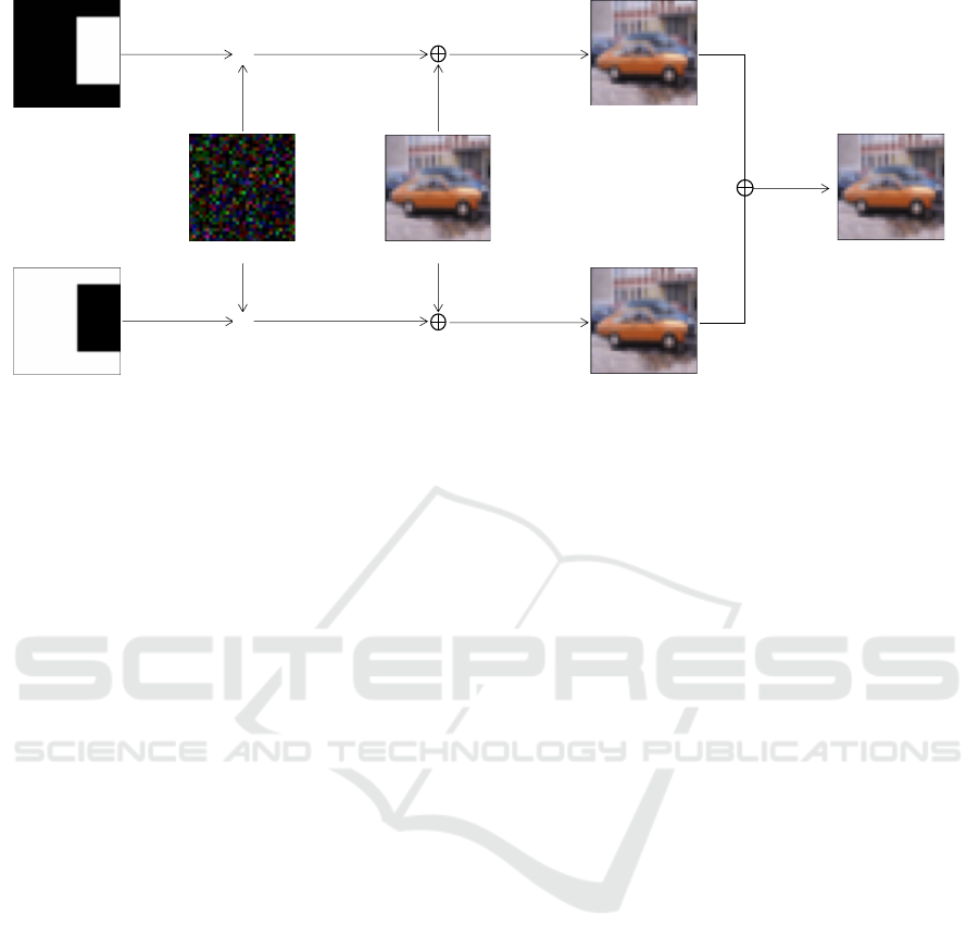
Figure 1 show the conceptual diagram of M

AT,

and Algorithm 1 is the pseudo code of our process.

3.2 Masking Phase

In the masking phase, we extract only speciﬁc regions

of adversarial perturbation computed by Eq. 6 with

the binary mask M ∈ {0,1}

h×w

, and create partially

perturbed images by applying extracted perturbation

to clean samples x

= x

+ δ

⊙ M, (7)

= x

+ δ

⊙ (1 − M), (8)

where, ⊙ is element-wise multiply. Following to Cut-

Mix (Yun et al., 2019), we compute the bounding box

coordinates B = (r

) for extracting the

perturbation with arbitrary probability λ

∼ U [0,1]:

Algorithm 1: Masking and Mixing Adversarial Training.

Require: Training dataset D, batch size n, training

epochs T, learning rate η, model parameter θ

θ,

hyper-parameter of beta distribution α

Require: The function deriving adversarial perturba-

tion A

Require: Masking function φ

1: for t = 1, . . . , T do

2: for {x

|i = 1,. . . , n} ∼ D do

← A(x

;θ

θ)

4: δ

←

− x

, λ

∼ U [0,1]

5: data masking and label smoothing phase:

6: ξ

← φ(

,δ

,λ

), λ

∼

Beta(α,α)

7: data mixing phase:

← λ

+ (1 − λ

)

← λ

+ (1 − λ

)

10: model update:

11: θ

t+1

← θ

− η ·

∑

i=1

∇

L( f

(

)

12: end for

13: end for

14: return model parameter θ

∼ U[0,W ], r

= min



W,W

1 − λ

+ r



, (9)

∼ U[0, H], r

= min



H,H

1 − λ

+ r



, (10)

where H and W are respectively height and width of

images. Note, both r

and r

sampled from U[0,W ]

and U[0, H] are not real number R but integer greater

than 0, i.e., Z

≥0

. We eventually get the binary mask

M as follows:

M =

(

1 if r

< M

:, j

< r

< M

i,:

< r

0 otherwise.

(11)

There is an inverse relation between ξ

and

: i.e.,

with/without the perturbed region is the same.

The ground truth label to perturbed images ob-

tained by these processes does not directly use λ

;

rather, we deﬁne smoothed labels with the area

ratio between clean and perturbed regions λ

′

(

−r

)

(

−r

)

H×W

= λ

′

+ (1 − λ

′

)

s, (12)

= λ

′

s + (1 − λ

′

, (13)

where y

represents a one-hot vector and

is all one

vector except true class y

(i.e., 1 − y

). s

s is a uniform

distribution assigned uniform probability 1/K − 1 to

all class except for true class y

3.3 Mixing Phase

AVmixup creates perturbed images by interpolat-

ing clean images and adversarial vertex samples

VISAPP 2023 - 18th International Conference on Computer Vision Theory and Applications

! ∈ {0, 1}

!×#

(

Perturbation Input image

Partial perturbed

image

Partial perturbed

image

Adversarial example

×*+

×*1* − *+

Partially perturbed

image

Partially perturbed

image

⊙

Figure 1: Conceptual diagram of computing adversarial examples for M

AT. Our method separates the perturbation with

binary masks, and we mix these two types of adversarial samples stochastically. M is a binary mask with a positive value (i.e.

1), for inside the rectangle.

M represents the contrasting binary mask for M. ⊙ and ⊕ represent element-wise multiply and

sum, respectively. λ

is the interpolation ratio and samples from Beta(α,α).

with an arbitrary interpolation ratio sampled from

Beta(1,1) = U[0, 1]. However, AVmixup is it limited

in terms of the amount of perturbed image variations

because they have a uniformly perturbed magnitude

over all the images.

Since we attempt to reduce the trade-off by aug-

menting the perturbed image variation, our method

uses the mixing phase for synthesizing two samples

computed in the masking phase. In the mixing phase,

we apply the perturbation to the entire image by mix-

ing two attacked images with an arbitrary interpola-

tion ratio, inspired by mixup (Zhang et al., 2018).

Note that perturbed images obtained via our method

have two types of perturbation magnitude in a single

image.

Let λ

∼ Beta(1,1). We then represent mixed

sample

and ground truth label

as follows:

= λ

+ (1 − λ

)

, (14)

= λ

+ (1 − λ

)

. (15)

This perturbed image is the same as AVmixup

with γ = 1 when λ

in the masking phase is 0 or 1.

We hope to improve the robustness by enabling the

model to train with a richer variation of adversarial

examples than AVmixup.

4 RELATED WORK

(Szegedy et al., 2014) is the ﬁrst work that han-

dled the vulnerability of CNNs to malicious noise,

called adversarial examples. Adversarial attack

methods for attacking CNNs have since been pro-

posed using various processes. (Goodfellow et al.,

2015)(Moosavi-Dezfooli et al., 2016)(Carlini and

Wagner, 2017)(Madry et al., 2018) derive adversar-

ial perturbations with the model gradients. These

attack methods presuppose a situation in which the

model parameters are known and are therefore called

white-box attacks. In contrast, the attack methods

for situations with unknown model parameters are

called black-box attacks. Papernot et al. is a well-

known black-box attack that deals with the transfer-

based threat of adversarial examples (Papernot et al.,

2016a). (Moosavi-Dezfooli et al., 2017) proposed

universal adversarial examples that do not decide the

perturbation for each sample but can induce misclas-

siﬁcation of multiple samples with only one perturba-

tion.

A model without countermeasures against adver-

sarial examples can fool even state-of-the-art models.

Adversarial defense studies are being actively con-

ducted to resolve this weakness and various power-

ful methods have been proposed. (Goodfellow et al.,

2015)(Madry et al., 2018)(Tram

er et al., 2018)(Wang

and Zhang, 2019)(Zhang and Wang, 2019) guarantee

model robustness by updating the model parameters

with adversarial examples. These methods have been

known adversarial training. (Papernot et al., 2016b)

is a defense method with knowledge distillation that

makes deriving the gradient difﬁcult by controlling

the temperature of the softmax function. (Meng and

Chen, 2017)(Samangouei et al., 2018) are defensive

techniques that prevent performance corruption by re-

Masking and Mixing Adversarial Training

moving the perturbation as much as possible from the

sample after inputting a classiﬁer.

5 EXPERIMENT

We compare our method with several previous works

to evaluate its defensive performance. We use

CIFAR-10/-100 as training datasets. CIFAR-10 is a

natural image dataset with ten classes of 32 ×32 RGB

data consisting of 50,000 training samples and 10,000

test samples. Each class has 5,000 samples for train-

ing and 1,000 samples for testing. CIFAR-100 is al-

most the same as CIFAR-10 except it has 100 classes,

with 500 training samples and 100 test samples in

each class.

5.1 Implementation Details

We use WRN34-10 (Wide Residual Net-

works) (Zagoruyko and Komodakis, 2016) on

both CIFAR-10 and CIFAR-100. The model trains

200 epochs (80,000 iterations) with a batch size of

128. The optimizer at training uses momentum SGD

with learning rate 0.1, momentum 0.9, and weight

decay 2.0 × 10

−4

. The learning rate is a factor of

0.1 at 50% and 75% for the number of epochs on

CIFAR-10.

Training samples use random crop and horizontal

ﬂip as data augmentation and the normalization range

[0, 1] for each pixel. We use the number of rounds k =

10, epsilon budget ε = 8, and step size α = 2 for PGD

during our training. We divide by 255 for each pixel

because both ε and α need to ﬁt the training sample

scale.

We evaluate the robustness of the trained model

with FGSM (Goodfellow et al., 2015), PGD (Madry

et al., 2018), and Carlini & Wagner (CW) (Carlini and

Wagner, 2017) as adversarial attack methods. k of

PGD-k and CW-k represents the number of rounds

for deriving adversarial examples. We compare our

method with the methods below.

• Standard: the model trained with standard training

data only.

• PGD: the PGD-trained model with number of

rounds k = 10 and ε = 8/255, α = 2/255.

• PGD with LS: the PGD-trained model with label

smoothing. A smoothing parameter samples from

Beta(1,1) during training.

• AVmixup: the model trained with the same set-

tings as (Lee et al., 2020).

100

1 51 101 151

Accuracy (%)

training epochs

100

1 51 101 151

Accuracy (%)

training epochs

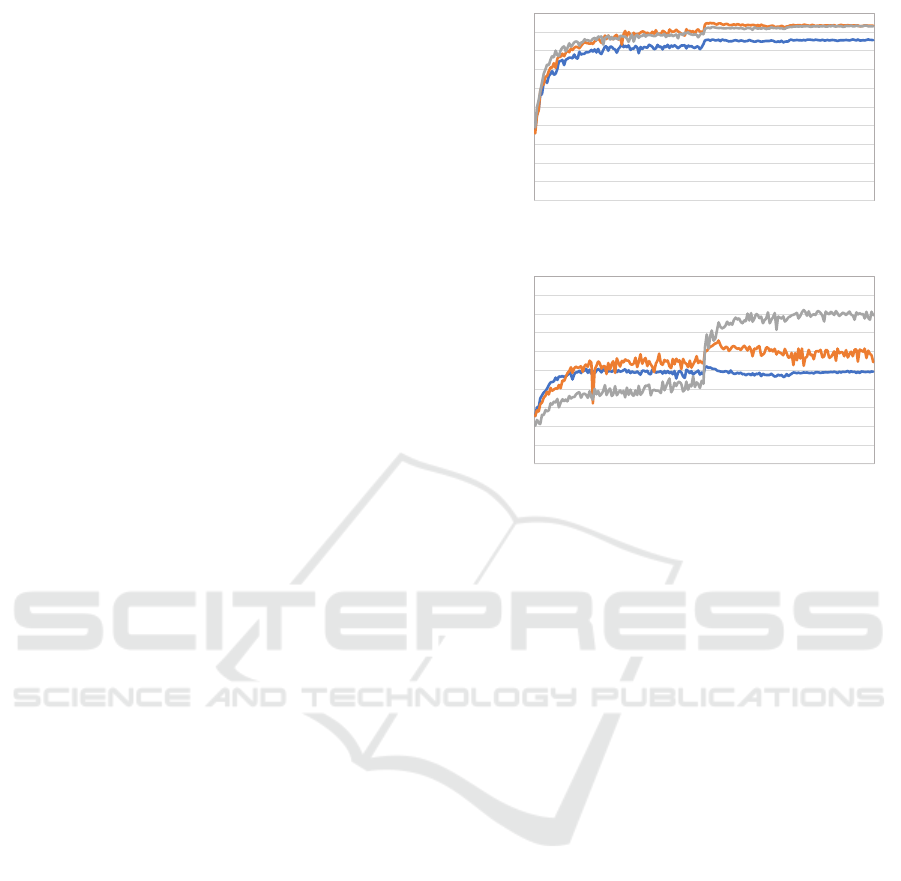
(a) Standard accuracy

(b) Adversarial robustness

Figure 2: Test accuracy transitions during training of clean

data and adversarial examples. The perturbation for adver-

sarial example derives by PGD with 10 rounds. Blue lines

are PGD, orange lines are AVmixup of our implementation,

and gray lines are M

AT.

Experimental results for all methods show the best

model, i.e., the highest-robustness model against

PGD-20 within training epochs, performance.

5.2 Comparison Results

The results on CIFAR-10 are listed in Table 1.

AT achieved a dramatic performance improvement

for the adversarial attack with FGSM and PGD-10/-

20. Its classiﬁcation accuracy to clean samples was

the same as that of AVmixup, and M

AT could pre-

vent extreme performance decreases. For the CW re-

sult, classiﬁcation performance only improved about

3%p from the AVmixup result. Both PGD-10 and -

20 with our method achived over 80% and improved

by about 30%p compared to PGD and by about 20%p

compared to AVmixup. As shown the gray line in

Figure 2(b), M

AT could avoid robust overﬁtting at

the same as AVmixup. The gap between accuracy and

robustness dramatically improved for several attacks

other than CW by using M

AT. Moreover, the re-

sult that ﬁt the base model to BAT (Wang and Zhang,

2019) outperformed BAT in terms of both clean accu-

racy and robustness.

In Table 1, all methods except ours had a gap of

about 10%p between FGSM and PGD-10/-20 accu-

VISAPP 2023 - 18th International Conference on Computer Vision Theory and Applications

Table 1: Comparison of classiﬁcation accuracy to clean data and robustness for adversarial attack with various methods. PGD

with LS represents PGD results using label smoothing with dynamic smoothing parameter. Results with * are those referenced

from original articles.

Dataset Model Clean FGSM PGD-10 PGD-20 CW-20

CIFAR-10

Standard 95.48 7.25 0.0 0.0 0.0

PGD 85.83 58.66 52.09 50.80 30.16

PGD with LS 86.33 61.67 55.87 54.78 30.36

BAT (Wang and Zhang, 2019)* 91.2 70.7 – 57.5 56.2

AVmixup* 93.24 78.25 62.67 58.23 53.63

AVmixup 94.81 80.28 69.29 65.01 54.8

AT (WRN28-10) 92.09 73.67 65.83 63.06 55.04

AT 93.16 83.35 82.29 80.66 56.90

CIFAR-100

PGD 61.29 46.01 – 25.17 –

AVmixup* 74.81 62.76 – 38.49 –

AVmixup 71.42 53.90 29.04 27.05 19.80

AT 69.14 32.63 32.63 29.99 18.48

Table 2: Accuracy comparison with TRADES on CIFAR-

10.

Clean PGD-20

PGD 87.3 47.04

TRADES (1/λ = 1) 88.64 49.14

TRADES (1/λ = 6) 84.92 56.61

AVmixup 90.36 58.27

AT 89.35 69.76

racy. In contrast, our method had hardly any gap be-

tween the two. We discuss this phenomenon in detail

in subsection 5.4.

The results on CIFAR-100 in Table 1 were no

better result than the AVmixup results in (Lee et al.,

2020), but our method performed better than our im-

plemented AVmixup. We could not obtain as good

a result as the previous work even when we changed

the ofﬁcial implementation on CIFAR-10

to CIFAR-

100 and trained. When we compare the results of

PGD and our method, FGSM was comparable and the

clean sample and PGD-20 improved by about 7%p

and 10%p, respectively. This demonstrates that our

method is better able to close the gap between accu-

racy and robustness than PGD.

Table 2 shows a performance comparison of our

method with TRADES, a defense method with reg-

ularization. While our method could not achieve as

good a result as AVmixup based on TRADES, but

PGD-20 improved by 10%p. Moreover, we could bet-

ter mitigate the gap between clean accuracy and ro-

bustness against perturbed images than AVmixup.

The ofﬁcial implementation of AVmixup:

https://github.com/Saehyung-Lee/cifar10 challenge

Table 3: Ablation results of our method.

Masking Mixing LS Clean FGSM PGD-20

✓ 86.33 61.67 54.78

✓ 89.60 54.75 44.70

✓ ✓ 93.97 74.81 60.96

✓ 89.92 56.36 43.72

✓ ✓ 93.36 65.80 42.46

✓ ✓ 90.21 60.14 49.25

✓ ✓ ✓ 93.16 83.35 80.66

5.3 Ablation Study

Table 3 shows the classiﬁcation accuracy of our

method with combinations ablating every element,

such as masking, mixing, and label smoothing. We

use a dynamic value sampled from Beta(1,1) as the

smoothing parameter.

We can see here that our model achieved the same

accuracy as AVmixup using just label smoothing. The

accuracy of PGD-20 was higher than that of AVmixup

thanks to creating perturbed images by combined la-

bel smoothing and mixing. This result is equal to

training AVmixup with γ = 1 except the smoothing

parameter is dynamic.

When training directly adversarial samples with

partially applied perturbation using a binary mask, the

performance with regards to robustness was inferior

to PGD (Table 1), but the accuracy to clean samples

slightly improved. This result suggests that we can

mitigate the trade-off by absorbing the frequency dif-

ferences for the clean and adversarial samples with

the model. The same tendency was evident when in-

terpolating adversarial examples and clean samples.

Partially perturbed images further improved the

clean accuracy and robustness against FGSM by train-

ing using label smoothing, but the PGD-20 result was

almost the same. On the other hand, the accuracy

Masking and Mixing Adversarial Training

100

8 16 32 64 128

100

8 16 32 64 128

100

8 16 32 64 128

PGD

AVmix u p

Accuracy (%)

𝜖 -budget 𝜖 -budget

𝜖 -budget

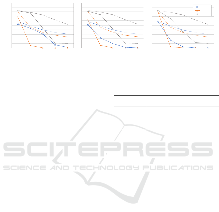
Figure 3: Accuracy transitions for adversarial examples at each ε budget. From left to right graphs are α = {2.0, 4.0,8.0}.

Solid and dashed lines are PGD-10 and FGSM, respectively, and each method is differentiates by color. FGSM accuracy in

all graphs was the same.

of PGD improved by linearly interpolating two par-

tially perturbed images, but others results, such as

clean and FGSM, suffered a decreased performance.

Overall, these results demonstrate that our method is

optimal for improving robustness against adversarial

examples and maintaining the performance for clean

samples.

5.4 Additional Discussion

FGSM vs. PGD for M

AT: Between PGD and

FGSM, we found that attacks caused a large gap be-

cause the adversarial examples created by PGD pro-

vide a more powerful threat than FGSM. On the

other hand, our method had only a small gap between

FGSM and PGD (Table 1). To clarify why this is so,

we investigate the accuracy transition when expand-

ing the budget size of the adversarial attack.

Figure 3 shows the accuracy transition for sought

perturbations with different budgets and step sizes

by FGSM and PGD-10. Although AVmixup could

achieve an excellent performance with ε-budget= 8,

its performance dramatically worsened for FGSM and

PGD-10 when it explored perturbation with a wide

budget over ε = 8. This indicates that AVmixup

cannot effectively defend against an adversarial at-

tack when the budget size expands to larger than that

used during training. While PGD did not experi-

ence so severe a collapse, it is still vulnerable to a

large ε-budget, the same as AVmixup. In contrast,

we can maintain a superior performance to the other

defense methods at all budget sizes. Moreover, our

method maintains a sufﬁcient performance up to ε-

budget= 32. Therefore, the model can handle a bud-

get size much larger than the one used during training

if it is trained using our method. According to these

results, AVmixup suffers from an overﬁt budget size

during training and its generalization performance is

extremely low, while our method generalizes to a dif-

ferent ε-budget. In other words, we believe that the

Table 4: Transfer-based black-box attack results (PGD-20).

The row methods are attack models and the column meth-

ods are defense models.

Defense

model

Attack model

PGD PGD with LS AVmixup

PGD – 50.83 50.86

PGD with LS 54.89 – 54.86

AVmixup 64.86 64.76 –

AT 80.77 80.62 80.82

model with AVmixup has many peak points outside

the ε-budget.

Black-Box Attack: We examine the robustness

against the transfer-based black-box attack, which at-

tacks the model with perturbations created by other

models. Since the white-box attack is an impossi-

ble situation, the black-box attack needs to be robust

against perturbation created without knowledge of the

parameters of the attack model. As shown in Table 4,

our method achieved the best performance against

perturbations created by any other models (e.g., PGD,

AVmixup). The demonstrate that the model trained

with our method is robust against perturbation created

by model gradients other than itself.

6 CONCLUSIONS

In this paper, we proposed Masking and Mixing Ad-

versarial Training, which can mitigate the trade-off

between accuracy and robustness by masking pertur-

bations with a binary mask and mixing them with an

arbitrary interpolation ratio. Experiments showed that

AT had a better performance than prior works on

the CIFAR-10 dataset and was robust against a large

ε-budget. While its performance on the CIFAR-100

dataset had the same accuracy as prior works, it could

not achieve state-of-the-art performance. This is be-

cause our adversarial examples were slightly differ-

ent from the original perturbations, which made the

VISAPP 2023 - 18th International Conference on Computer Vision Theory and Applications

model classiﬁcation is unstable when classes were in-

creased. We should be able to improve the perfor-

mance of our method on CIFAR-100 by developing

a better method for creating the ground truth label or

optimizing the training process. In future work, we

will theoretically investigate our method and improve

the training process.

ACKNOWLEDGEMENTS

This work was supported by JST SPRING, Grant

Number JPMJSP2158.

REFERENCES

Brock, A., Donahue, J., and Simonyan, K. (2019). Large

scale gan training for high ﬁdelity natural image syn-

thesis. In the International Conference on Learning

Representations.

Carlini, N. and Wagner, D. (2017). Towards evaluating the

robustness of neural networks. In the IEEE Sympo-

sium on Security and Privacy, volume 1, pages 39–57.

Goodfellow, I., Shlens, J., and Szegedy, C. (2015). Explain-

ing and harnessing adversarial examples. In the Inter-

national Conference on Learning Representations.

Guo, H., Mao, Y., and Zhang, R. (2019). Mixup as locally

linear out-of-manifold regularization. In the AAAI

Conference on Artiﬁcial Intelligence, volume 33,

pages 3714–3722.

He, K., Zhang, X., Ren, S., and Sun, J. (2016). Deep resid-

ual learning for image recognition. In the IEEE Con-

ference on Computer Vision and Pattern Recognition,

pages 770–778.

Lee, S., Lee, H., and Yoon, S. (2020). Adversarial vertex

mixup-toward better adversarially robust generaliza-

tion. In the IEEE/CVF Conference on Computer Vi-

sion and Pattern Recognition, pages 272–281.

Long, J., Shelhamer, E., and Darrell, T. (2015). Fully con-

volutional networks for semantic segmentation. In

the IEEE Conference on Computer Vision and Pattern

Recognition, pages 3431–3440.

Madry, A., Makelov, A., Schmidt, L., Tsipras, D., and

Vladu, A. (2018). Towards deep learning models re-

sistant to adversarial attacks. In the International Con-

ference on Learning Representations.

Meng, D. and Chen, H. (2017). Magnet: a two-pronged de-

fense against adversarial examples. In the ACM Con-

ference on Computer and Communications Security,

pages 135—147.

Moosavi-Dezfooli, S.-M., Fawzi, A., Fawzi, O., and

Frossard, P. (2017). Universal adversarial perturba-

tions. In the IEEE Conference on Computer Vision

and Pattern Recognition, pages 1765–1773.

Moosavi-Dezfooli, S.-M., Fawzi, A., and Frossard, P.

(2016). Deepfool: a simple and accurate method

to fool deep neural networks. In 2574-2582, editor,

the IEEE Conference on Computer Vision and Pattern

Recognition.

Papernot, N., McDaniel, P., and Goodfellow, I. (2016a).

Transferability in machine learning: from phenomena

to black-box attacks using adversarial samples. arXiv

preprint arXiv:1605.07277.

Papernot, N., McDaniel, P., Wu, X., Jha, S., and Swami, A.

(2016b). Distillation as a defense to adversarial per-

turbations against deep neural networks. In the IEEE

Symposium on Security and Privacy.

Qin, J., Fang, J., Zhang, Q., Liu, W., Wang, X., and Wang,

X. (2020). Resizemix: Mixing data with preserved

object information and true labels. arXiv preprint

arXiv:2012.11101.

Redmon, J., Divvala, S., Girshick, R., and Farhadi, A.

(2016). You only look once: Uniﬁed, real-time ob-

ject detection. In the IEEE Conference on Computer

Vision and Pattern Recognition, pages 779–788.

Samangouei, P., Kabkab, M., and Chellappa, R. (2018).

Defense-gan: Protecting classiﬁers against adversarial

attacks using generative models. In the International

Conference on Learning Representations.

Schmidt, L., Santurkar, S., Tsipras, D., Talwar, K., and

Madry, A. (2018). Adversarially robust generaliza-

tion requires more data. In the Advances in Neural

Information Processing Systems.

Shafahi, A., Najibi, M., Ghiasi, A., Xu, Z., Dickerson, J.,

Studer, C., Davis, L. S., Taylor, G., and Goldstein, T.

(2019). Adversarial training for free! In the Advances

in Neural Information Processing Systems.

Szegedy, C., Vanhoucke, V., Ioffe, S., Shlens, J., and Wo-

jna, Z. (2016). Rethinking the inception architecture

for computer vision. In the IEEE Conference on Com-

puter Vision and Pattern Recognition, pages 2818–

2826.

Szegedy, C., Zaremba, W., Sutskever, I., Bruna, J., Erhan,

D., Goodfellow, I., and Fergus, R. (2014). Intrigu-

ing properties of neural networks. In the International

Conference on Learning Representations.

Tram

er, F., Kurakin, A., Papernot, N., Goodfellow, I.,

Boneh, D., and McDaniel, P. (2018). Ensemble ad-

versarial training: Attacks and defenses. In the Inter-

national Conference on Learning Representations.

Tsipras, D., Santurkar, S., Engstrom, L., Turner, A., and

Madry, A. (2019). Robustness may be at odds with

accuracy. In the International Conference on Learning

Representations.

Wang, J. and Zhang, H. (2019). Bilateral adversarial train-

ing: Towards fast training of more robust models

against adversarial attacks. In the IEEE/CVF Interna-

tional Conference on Computer Vision, pages 6629–

6638.

Wong, E., Rice, L., and Kolter, J. Z. (2020). Fast is better

than free: Revisiting adversarial training. In the Inter-

national Conference on Learning Representations.

Xie, C., Wang, J., Zhang, Z., Zhou, Y., Xie, L., and Yuille,

A. (2017). Adversarial examples for semantic seg-

mentation and object detection. In the IEEE Interna-

Masking and Mixing Adversarial Training

tional Conference on Computer Vision, pages 1369–

1378.

Yamanaka, K., Matsumoto, R., Takahashi, K., and Fujii,

T. (2020). Adversarial patch attacks on monocular

depth estimation networks. IEEE Access, 8:179094–

179104.

Yin, D., Lopes, R. G., Shlens, J., Cubuk, E. D., and Gilmer,

J. (2019). A fourier perspective on model robustness

in computer vision. In the Advances in Neural Infor-

mation Processing Systems.

Yun, S., Han, D., Oh, S. J., Chun, S., Choe, J., and Yoo,

Y. (2019). Cutmix: Regularization strategy to train

strong classiﬁers with localizable features. In the

IEEE/CVF International Conference on Computer Vi-

sion, pages 6023–6032.

Zagoruyko, S. and Komodakis, N. (2016). Wide residual

networks. arXiv preprint arXiv:1605.07146.

Zhang, H., Cisse, M., Dauphin, Y. N., and Lopez-Paz, D.

(2018). mixup: Beyond empirical risk minimization.

In the International Conference on Learning Repre-

sentations.

Zhang, H. and Wang, J. (2019). Defense against adversar-

ial attacks using feature scattering-based adversarial

training. In the Advances in Neural Information Pro-

cessing Systems, volume 32.

VISAPP 2023 - 18th International Conference on Computer Vision Theory and Applications