DNN Pruning and Its Effects on Robustness
Sven Mantowksy, Firas Mualla, Saqib Sayad Bukhari and Georg Schneider
ZF Friedrichshafen AG, AI-Lab, Saarbr
¨
ucken, Germany
Keywords:
Pruning, Explainability, Calibration.
Abstract:
The popularity of deep neural networks (DNNs) and their application on embedded systems and edge devices
is increasing rapidly. Most embedded systems are limited in their computational capabilities and memory
space. To meet these restrictions, the DNNs need to be compressed while keeping their accuracy, for instance,
by pruning the least important neurons or filters. However, the pruning may introduce other effects on the
model, such as influencing the robustness of its predictions. To analyze the impact of pruning on the model ro-
bustness, we employ two metrics: heatmap based correlation coefficient (HCC) and expected calibration error
(ECE). Using the HCC, on one hand it is possible to gain insight to which extent a model and its compressed
version tend to use the same input features. On the other hand, using the difference in the ECE between a
model and its compressed version, we can analyze the side effect of pruning on the model’s decision reliabil-
ity. The experiments were conducted for image classification and object detection problems. For both types of
issues, our results show that some off-the-shelf pruning methods considerably improve the model calibration
without being specifically designed for this purpose. For instance, the ECE of a VGG16 classifier is improved
by 35% after being compressed by 50% using the H-Rank pruning method with a negligible loss in accuracy.
Larger compression ratios reduce the accuracy as expected but may improve the calibration drastically (e.g.
ECE is reduced by 77% under a compression ratio of 70%). Moreover, the HCC measures feature saliency
under model compression and tends to correlate as expected positively with the model’s accuracy. The pro-
posed metrics can be employed for comparing pruning methods from another perspective than the commonly
considered trade-off between the accuracy and compression ratio.
1 INTRODUCTION
The popularity of deep neural networks (DNNs), es-
pecially convolutional neural networks, has increased
over the last few years. Their applications have be-
come indispensable in areas such as computer vision,
robotics (Brunke et al., 2022), natural language pro-
cessing (Otter et al., 2020) and optimization of indus-
trial processes (Weichert et al., 2019). For a while
now, neural networks can even outperform humans in
different tasks such as voice and object recognition,
which emphasizes their usability even more. How-
ever, to achieve such an outstanding performance,
neural networks are becoming more complex, leading
to over-parameterization and more computationally
expensive operations. This situation necessitates large
computational capacity, more memory and an overall
increase in power consumption. These complexities
impede the transition of a deep learning model into
a product-level application, especially when embed-
ded systems or edge devices are used. In particular,
the automotive field has strict requirements regarding
computationally expensive algorithms such as deep
learning models. For this reason, researchers are in-
vestigating various pruning methods to reduce the size
of neural networks. The most common approach is
to identify and to remove the least important network
components, while avoiding any adverse effect on
overall accuracy. This sort of model’s compression
enables the deployment of large deep learning models
on resource-constrained edge devices. Most pruning
algorithms focus only on simple key performance in-
dicators (KPI), such as accuracy and inference time
after pruning. However, these KPIs cannot provide a
deeper insight into other changes introduced by prun-
ing, such as regarding model robustness.
To resolve this problem, we present two met-
rics to analyze the robustness of compressed mod-
els. The first metric uses the correlation between a
pair of heatmaps, generated for an input sample for
the model and its pruned version. With the help of
these heatmaps, we can evaluate which features are
decisive for a prediction. Comparing two different
heatmaps of an unpruned and pruned model can show
if the areas of interest change after pruning. It is
called Heatmap Correlation Coefficient (HCC). The
82
Mantowksy, S., Mualla, F., Bukhari, S. and Schneider, G.
DNN Pruning and Its Effects on Robustness.
DOI: 10.5220/0011651000003411
In Proceedings of the 12th International Conference on Pattern Recognition Applications and Methods (ICPRAM 2023), pages 82-88
ISBN: 978-989-758-626-2; ISSN: 2184-4313
Copyright
c
 2023 by SCITEPRESS – Science and Technology Publications, Lda. Under CC license (CC BY-NC-ND 4.0)

heatmaps are generated using Deep Taylor Decompo-
sition (DTD) method (Montavon et al., 2017b). Since
the original version of DTD is limited to image classi-
fication problem, we use a further developed in-house
version of the DTD method for object detection. The
second metric employs miscalibration measurement,
particularly Expected Calibration Error (ECE) (Guo
et al., 2017). In order to compare the calibration of a
pruned model with its unpruned baseline we use re-
liability diagrams to measure the changes in the re-
lationship between accuracy and output’s confidence.
We summarize our contributions as follows:
• We employ heatmaps to measure feature saliency
under pruning using HCC.
• We show through experiments with ECE and re-
liability diagrams that pruned models can be con-
siderably better in calibration as compared to un-
pruned models, even without using a pruning
method specifically designed for this purpose.
• The proposed metrics are flexibly applicable to
off-the-shelf pruning techniques and models, al-
lowing very versatile applicability.
2 RELATED WORK
There have been frequent reports in literature empha-
sizing the role of pruning in improving the generaliz-
ability of neural networks to unseen examples (LeCun
et al., 1989; Hassibi and Stork, 1992; Hoefler et al.,
2021; Nadizar et al., 2021).
Recently, researchers (Jord
˜
ao and Pedrini, 2021;
Guo et al., 2018) showed that pruning tends also to
improve the adversarial robustness of the resulting
models even without adversarial training. The pruned
models therefore tend not to inherit the adversarial
vulnerability of the original models. Some other ap-
proaches combine both adversarial training and prun-
ing to maximize robustness (Ye et al., 2019; Sehwag
et al., 2020; Gui et al., 2019). This line of work
has also been extended to the so-called certifiably ro-
bust approaches against adversarial attacks (Li et al.,
2022). For these types of methods, usually, either the
pruning procedure or the training is modified to im-
prove adversarial robustness.
The works mentioned above studied the positive
side effects of pruning on the robustness defined in
terms of generalizability to unseen examples or im-
munity to adversarial attacks. In this work, however,
we are interested in robustness in terms of model cal-
ibration and model-side feature saliency for off-the-
shelf pruning methods.
3 METHODS
3.1 Neural Network Pruning
Pruning methods reduce the size of an already trained
model to correspondingly decrease the runtime, mem-
ory footprint, and power consumption. For this pur-
pose, redundant parameters are removed from the
model while trying to preserve the model accuracy
compared to the baseline model. Since pruning has
a regularization effect (Bartoldson et al., 2020), it is
sometimes even possible to gain some improvement
in accuracy by pruning, especially when the initial
network is over-parameterized.
In general, pruning methods can be divided into
two main categories: structured and unstructured
pruning. In structured pruning, complete structures
such as layers (Wang et al., 2017), filters (Zeng and
Urtasun, 2019) or channels (He et al., 2017) are re-
moved. On the other hand, in unstructured prun-
ing (Lee et al., 2018; Kwon et al., 2020), individual
weights are set to zero (Han et al., 2015; Hayou et al.,
2021). Unstructured pruning methods suffer signif-
icant drawbacks, such as particular frameworks and
chip architectures are required, as not all algorithms
and hardware architectures can exploit weight spar-
sity to improve performance. Therefore, in this work
we consider only structured pruning methods for our
experiments.
3.2 Heatmap Generation Using Deep
Taylor Decomposition
While being known to perform very well at least
for in-distribution data, deep neural networks tend to
show a kind of black-box behavior compared to other
more transparent machine learning paradigms such as
simple linear classifiers or decision trees. Explainable
Artificial Intelligence (XAI) (Arrieta et al., 2020) is
a relatively new field that addresses this black-box-
behavior issue. Deep Taylor Decomposition (DTD)
(Montavon et al., 2017a) is an XAI method inspired
by decomposing a function value (e.g. object score
or class probability) as a sum of input feature con-
tributions based on the Taylor series. The relevance
R of a neuron inside a layer l of a neural network is
decomposed in terms of the activations a of the pre-
vious layer l − 1. More specifically, a root a
0
of the
relevance R in the space of the activations of the previ-
ous layer must be first found. A linear approximation
of Taylor expansion of R can be then computed as the
inner product of (a − a
0
) and the gradient of R at a
0
.
This inner product is a sum of terms, each of them
contributes to calculating the relevance of a neuron in
DNN Pruning and Its Effects on Robustness
83

Input
bird
Baselin e
bird
HCC:0.97
Compression : 25%
bird
HCC:0.91
Compression : 50%
Input
person
Baselin e
person
HCC:0.85
Compression : 25%
person
HCC:0.64
Compression : 50%
Figure 1: DTD Heatmaps are generated for each object in the image (one object per figure’s row). Columns show from left
to right: input image of the object detector SSD, heatmap of the unpruned model, heatmap of the model pruned by 25%, and
heatmap of the model pruned by 50%. The HCC (see text) measures the feature saliency under model compression.
the previous layer l − 1 based on the relevance of the
considered neuron in layer l. The method is closely
related to another XAI method called Layerwise Rel-
evance Propagation (LRP) (Bach et al., 2015). The
LRP is a scheme of different propagation rules for the
redistribution of a neuron’s relevance on the neurons
of its previous layer. In particular, the so-called LRP
γ-rule can be given as follows:
R
i
=
∑
j
z
i j
+ γz
+
i j
ε +
∑
k
z
k j
+ γz
+
k j
R
j
, (1)
z
i j
= a
i
w
i j
(2)
z
+
i j
= max(0, z
i j
) (3)
where R
j
denotes the relevance of a neuron j, w
i j
the
weight connecting neuron i with neuron j, a
i
the acti-
vation of the neuron i, ε is an arbitrary small number,
and γ is a parameter of the rule.
Under the assumption of a relu activation function,
the DTD is equivalent to the LRP γ-rule when γ → ∞
(Samek et al., 2021). This equivalence was employed
to simplify the implementation of the DTD. Both the
DTD and LRP are originally designed for image clas-
sification problems. For this work, we used an exten-
sion of DTD that can be applied to both classification
and object detection problems (KIA Project Booklet,
2022).
3.3 Heatmap Correlation Coefficient
We employ the heatmap concept to assess feature
saliency under pruning. The correlation coefficient
between the heatmap of the baseline model H
b
and
the heatmap of the pruned model H
p
is computed as
follows:
HCC(H
b
, H
p
) =
1
n
∑
i, j
(H
b
(i, j)−µ
H
b
)(H
p
(i, j)−µ
H
p
)
σ
H
b
σ
H
p
, (4)
where n is the number of pixels, µ
H
b
, σ
H
b
, µ
H
p
, σ
H
p
are the mean and standard deviation of the baseline
and the pruned models, respectively. Figure 1 demon-
strates the calculation of HCC using DTD heatmaps
applied to object detection.
3.4 Expected Calibration Error (ECE)
To evaluate the performance of a deep learning model,
accuracy is often insufficient, as the confidence of a
model’s decision and not only the decision itself has
to be evaluated. Reliability diagrams are usually em-
ployed to measure the deviation between the model’s
confidence and measured accuracy. The identity func-
tion would represent a perfect calibration (shown as a
dashed line in the ECE figures below). Any deviation
from this identity function means a miscalibration of
the model, and the model is considered accordingly
either overconfident or underconfident. The confi-
dence in this scenario is represented by the models
probability outputs. Inside each small interval (bin)
B
m
of the confidence, the deviation between measured
accuracy acc(B
m
) inside this bin and the center of the
bin con f (B
m
) can be calculated. The expected cali-
bration error is defined as the expectation (weighted
sum) of these deviations:
ECE =
M
∑
m=1
|
B
m
|
S
|
acc(B
m
) − con f (B
m
)
|
, (5)
where
|
B
m
|
is the number of samples inside the bin, M
is the number of bins, and S is the number of samples.
ICPRAM 2023 - 12th International Conference on Pattern Recognition Applications and Methods
84

10 20 30 40 50 60 70 80
P runing ratio [%]
0.0
0.2
0.4
0.6
0.8
1.0
HCC
Hrank
L1 norm
SF P
0
20
40
60
Accuracy [%]
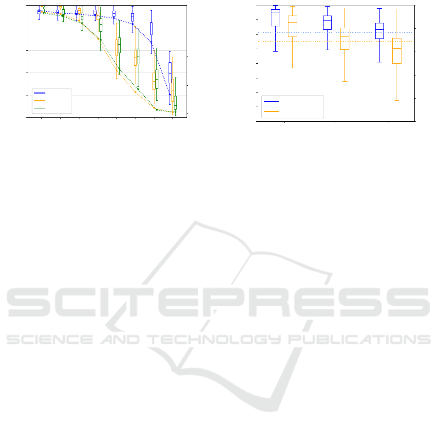
Figure 2: Boxplot of HCC of heatmap pairs for the VGG16,
compressed with different pruning methods and compres-
sion ratios. The dotted lines show the accuracy of each
pruned model at the corresponding pruning ratio. The box-
plots are grouped to a compression rate of 10%.
In some contexts, especially in safety-critical appli-
cations, the maximum deviation between confidence
and accuracy can be additionally considered:
MCE = max
m∈
{
1,...,M
}
|
acc(B
m
) − con f (B
m
)
|
. (6)
4 RESULTS
In this Section, we present the results of heatmap cor-
relation and the impact of pruning on network cali-
bration. We distinguish between classification using
the VGG16 model (Simonyan and Zisserman, 2014)
and object detection using the Single Shot Detector
(SSD) (Liu et al., 2016). For classification, we used
three different pruning methods: L1-norm (Li et al.,
2016), HRank (Lin et al., 2020) and Soft Filter Prun-
ing (SFP) (He et al., 2019). For object detection, we
extended the HRank method to be applicable to all
layers of the SSD.
4.1 Heatmap Correlation
In Section 3.3, we introduced the heatmap correlation
coefficient (HCC) as a metric to analyze the impact of
pruning using the heatmap methods. First, we present
the results of the classification model VGG16, pruned
with three different pruning methods and compression
rates between 0% and 80%. Higher compression rates
are negligible as the accuracy already drops to less
than 5% for a compression rate of 80%. The results
are visualized as a boxplot in Figure 2. The trend of
HCC over different compression ratios seems to be
very similar for all pruning methods. However, on
closer inspection, it becomes apparent for L1-norm
and SFP, that the HCC decreases continuously as the
S M L
Instance Size
0.80
0.83
0.85
0.88
0.90
0.93
0.95
0.98
1.00
HCC
0
20
40
60
80
100
Accuracy [%]
25% Pruning
50% Pruning
Figure 3: Distribution of HCC for the SSD, compressed
with the HRank method with two different compression
rates, categorized by object sizes. The dotted line shows
the accuracy of each model. The PASCAL VOC dataset
was used for both experiments.
compression rate increases, which corresponds to ex-
pectations. The HCC of the HRank method, how-
ever, remains almost constant up to a compression
rate of 55%, which indicates a more robust network
and therefore a more robust pruning method.
As mentioned above, we adapted the HRank
method to work with all layers of the SSD. After train-
ing the SSD on the PASCAL VOC dataset, we made
sure that the extended HRank pruning was working
fine. We were able to compress the model by up to
50%. We generated heatmap pairs under the same
procedure described above, with the addition that we
categorized the resulting bounding boxes according to
object size. This is based on the categorization of the
PASCAL VOC dataset, in which the difficulty of an
object depends, among other criteria, on its size. The
distribution of all HCC results for compression ratios
of 25% and 50% are shown in Figure 3. A decrease in
the HCC can be clearly seen as the compression rate
increases and this reflects the behavior of the classi-
fication results shown previously. The difference in
HCC between the 25% and 50% compressed model
can also be seen more clearly for large objects. In
case of large instances, it is more common for struc-
tures in the background to contribute slightly to the
result. After pruning, the probabilities of contribut-
ing background pixels can increase which leads to a
decrease in HCC. Figure 1 (2
nd
row) shows such an
example, in which the probabilities of the background
structures increase with the compression ratio.
4.2 Network Calibration
The calibration error is an additional tool to evaluate
the change in robustness after pruning compared to
its baseline. The ECE is a suitable metric for this pur-
DNN Pruning and Its Effects on Robustness
85

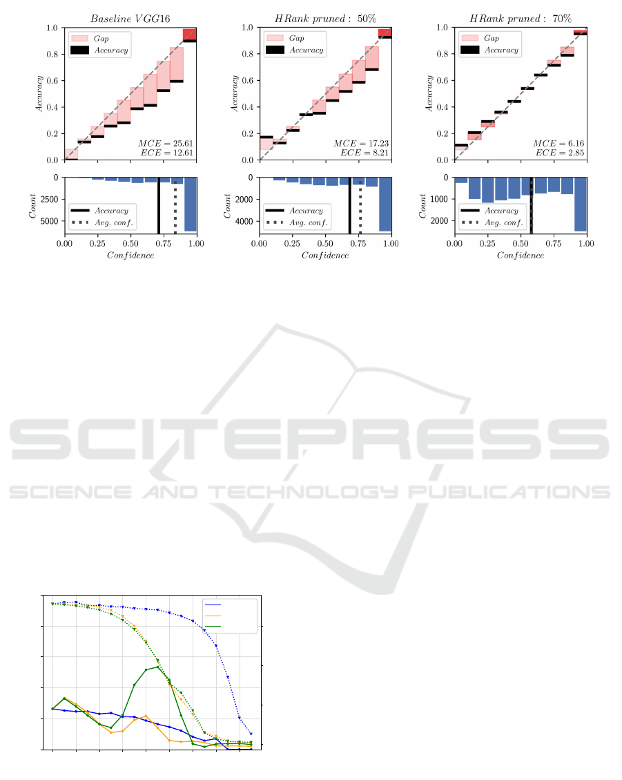
Figure 5: Reliability diagrams of VGG16: (a) unpruned model, (b) pruned with HRank method and a compression ratio of
50%, (c) pruned with HRank method and a compression ratio of 70%. The dotted line in the upper graph represents the perfect
calibration. The lower graph represents the number of objects within an interval (bin).
pose, as described in Section 3.4. First, we present
the results of the VGG16 model pruned with HRank,
L1-norm, and SFP before proceeding to object detec-
tion. The baseline is the VGG16 trained on the CI-
FAR100 dataset, with an accuracy of 71.26%. While
increasing the compression rate, the accuracy begins
to decrease, but a significant loss for L1-norm and
SFP can first be seen from 25% compression rate and
for HRank from 55% compression rate onward. The
ECE was calculated for each model after pruning and
is shown in Figure 4. Two aspects stand out:
(i) It can be clearly seen that pruning has a posi-
tive effect on the calibration of a network. Often, at
meager compression rates, accuracy even increases,
giving an additional advantage through pruning. At
higher compression rates, there is a trade-off between
0 10 20 30 40 50 60 70 80
P runing ratio[%]
0.0
10.0
20.0
30.0
40.0
50.0
Expected Calibration Error
Hrank
L1 norm
SF P
0
20
40
60
Accuracy [%]
Figure 4: Comparing Expected Calibration Error for differ-
ent compression ratios (0% - 85%) after pruning the VGG16
with three different pruning methods (HRank, L1 norm and
SFP). The dotted line shows the accuracy of each pruned
model at the corresponding pruning ratio. The sampling
rate of the compression rate is 5%.
accuracy and calibration that must be considered in-
dividually.
(ii) For L1-norm and SFP, with a substantial de-
crease in accuracy, the ECE also increases rapidly
(from 25% compression rate onwards), until the accu-
racy converges towards zero. In this point, the HRank
method differs from the other two methods, although
the reason needs to be investigated.
For a better understanding of the calibration, a re-
liability diagram with the values of ECE is shown in
Figure 5 for a better understanding of the calibration
and the value of the ECE. Compared to the baseline,
the accuracy of the 50% pruned model is reduced only
by 2.14%. However, the ECE has improved by 35%
from 12.61 of the baseline. This is an unambigu-
ous indication that pruning can impact and improve a
network’s decision and therefore making it safer and
more robust. Further pruning as seen in Figure 5 (c),
yields a drop in accuracy but improves model calibra-
tion. It thus improves the model’s awareness of its
low accuracy.
We applied the same procedure to object detec-
tion. However, due to the high expenditure of time
for implementation and testing, we have limited our-
selves to the HRank method. Figure 6 shows the re-
sult of an SSD pruned by a compression rate of 25%.
Compared to image classification problem, there is no
confidence below 0.3, as this limit is the minimum to
accept a prediction final detection. As before, the re-
sult shows an improvement in ECE of nearly 10%,
while the detector’s accuracy decreases by less than
1%. Thus, pruning improves the calibration of object
detection models as well.
ICPRAM 2023 - 12th International Conference on Pattern Recognition Applications and Methods
86

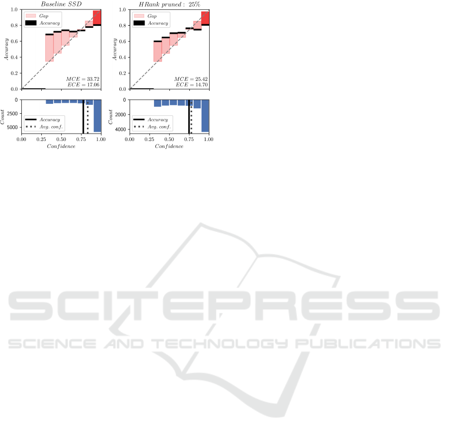
(a) (b)
Figure 6: Reliability diagram of SSD (a) unpruned and
(b) pruned with HRank method and a compression ratio of
25%. The graph shows no calibration for confidences less
than 0.3, since the confidence threshold for a detection is
set to 0.3, based on the original publication of the SSD. The
dotted line in the upper graph represents the perfect cali-
bration. The lower graph represents the number of objects
within an interval (bin).
5 CONCLUSIONS
In this paper we analyzed some side effects of off-the-
shelf pruning methods on both model calibration and
feature saliency. Our results show that pruning may
considerably improve the model’s calibration without
being specifically designed for this purpose. A well-
calibrated model excels at estimating the reliability of
its own decisions. Pruning may thus have a positive
effect on reliability and robustness. This result com-
plements literature reports pointing out a positive con-
tribution of the pruning to adversarial robustness.
Additionally, we employ heatmap methods from
the field of XAI, particularly the similarity between
the heatmap of a pruned model and the heatmap of its
unpruned baseline to investigate the effects of prun-
ing on feature saliency. As expected, pruned models
tend to look at features differently than those being
considered by the unpruned baseline when the accu-
racy drops. Therefore it makes sense in future work to
enforce a kind of heatmap saliency in the model com-
pression process to improve the accuracy of pruned
models.
ACKNOWLEDGEMENTS
The research leading to these results was partially
funded by the German Federal Ministry for Eco-
nomic Affairs and Energy within the project
”KI-Absicherung” (grant: 19A19005U).
REFERENCES
Arrieta, A. B., D
´
ıaz-Rodr
´
ıguez, N., Del Ser, J., Bennetot,
A., Tabik, S., Barbado, A., Garc
´
ıa, S., Gil-L
´
opez, S.,
Molina, D., Benjamins, R., et al. (2020). Explainable
artificial intelligence (xai): Concepts, taxonomies, op-
portunities and challenges toward responsible ai. In-
formation fusion, 58:82–115.
Bach, S., Binder, A., Montavon, G., Klauschen, F., M
¨
uller,
K.-R., and Samek, W. (2015). On pixel-wise explana-
tions for non-linear classifier decisions by layer-wise
relevance propagation. PLoS ONE, 10(7):e0130140.
Bartoldson, B. R., Morcos, A. S., Barbu, A., and Er-
lebacher, G. (2020). The generalization-stability
tradeoff in neural network pruning.
Brunke, L., Greeff, M., Hall, A. W., Yuan, Z., Zhou, S.,
Panerati, J., and Schoellig, A. P. (2022). Safe learn-
ing in robotics: From learning-based control to safe
reinforcement learning. Annual Review of Control,
Robotics, and Autonomous Systems, 5:411–444.
Gui, S., Wang, H., Yang, H., Yu, C., Wang, Z., and Liu, J.
(2019). Model compression with adversarial robust-
ness: A unified optimization framework. Advances in
Neural Information Processing Systems, 32.
Guo, C., Pleiss, G., Sun, Y., and Weinberger, K. Q. (2017).
On calibration of modern neural networks. In Interna-
tional conference on machine learning, pages 1321–
1330. PMLR.
Guo, Y., Zhang, C., Zhang, C., and Chen, Y. (2018). Sparse
dnns with improved adversarial robustness. Advances
in neural information processing systems, 31.
Han, S., Pool, J., Tran, J., and Dally, W. J. (2015). Learn-
ing both weights and connections for efficient neu-
ral networks. In Proceedings of the 28th Interna-
tional Conference on Neural Information Processing
Systems - Volume 1, NIPS’15, page 1135–1143, Cam-
bridge, MA, USA. MIT Press.
Hassibi, B. and Stork, D. (1992). Second order deriva-
tives for network pruning: Optimal brain surgeon. Ad-
vances in neural information processing systems, 5.
Hayou, S., Ton, J.-F., Doucet, A., and Teh, Y. W. (2021).
Robust pruning at initialization. In International Con-
ference on Learning Representations.
He, Y., Dong, X., Kang, G., Fu, Y., Yan, C., and Yang, Y.
(2019). Asymptotic soft filter pruning for deep con-
volutional neural networks. IEEE transactions on cy-
bernetics, 50(8):3594–3604.
He, Y., Zhang, X., and Sun, J. (2017). Channel pruning for
accelerating very deep neural networks. In 2017 IEEE
International Conference on Computer Vision (ICCV),
pages 1398–1406.
Hoefler, T., Alistarh, D., Ben-Nun, T., Dryden, N., and
Peste, A. (2021). Sparsity in deep learning: Pruning
and growth for efficient inference and training in neu-
ral networks. J. Mach. Learn. Res., 22(241):1–124.
DNN Pruning and Its Effects on Robustness
87

Jord
˜
ao, A. and Pedrini, H. (2021). On the effect of prun-
ing on adversarial robustness. In Proceedings of the
IEEE/CVF International Conference on Computer Vi-
sion (ICCV) Workshops, pages 1–11.
KIA Project Booklet (2022). KI Absicherung
Overview and Poster Abstracts. https:
//www.ki-absicherung-projekt.de/fileadmin/
KI Absicherung/Final Event/KI-A poster-booklet
Onlineversion.pdf.
Kwon, S. J., Lee, D., Kim, B., Kapoor, P., Park, B., and
Wei, G.-Y. (2020). Structured compression by weight
encryption for unstructured pruning and quantization.
In Proceedings of the IEEE/CVF Conference on Com-
puter Vision and Pattern Recognition, pages 1909–
1918.
LeCun, Y., Denker, J., and Solla, S. (1989). Optimal brain
damage. Advances in neural information processing
systems, 2.
Lee, N., Ajanthan, T., and Torr, P. H. (2018). Snip: Single-
shot network pruning based on connection sensitivity.
arXiv preprint arXiv:1810.02340.
Li, H., Kadav, A., Durdanovic, I., Samet, H., and Graf, H. P.
(2016). Pruning filters for efficient convnets. arXiv
preprint arXiv:1608.08710.
Li, Z., Chen, T., Li, L., Li, B., and Wang, Z. (2022). Can
pruning improve certified robustness of neural net-
works? arXiv preprint arXiv:2206.07311.
Lin, M., Ji, R., Wang, Y., Zhang, Y., Zhang, B., Tian, Y., and
Shao, L. (2020). Hrank: Filter pruning using high-
rank feature map. In Proceedings of the IEEE/CVF
conference on computer vision and pattern recogni-
tion, pages 1529–1538.
Liu, W., Anguelov, D., Erhan, D., Szegedy, C., Reed, S.,
Fu, C.-Y., and Berg, A. C. (2016). Ssd: Single shot
multibox detector. In European conference on com-
puter vision, pages 21–37. Springer.
Montavon, G., Lapuschkin, S., Binder, A., Samek, W., and
M
¨
uller, K.-R. (2017a). Explaining nonlinear classifi-
cation decisions with deep taylor decomposition. Pat-
tern Recognition, 65:211 – 222.
Montavon, G., Lapuschkin, S., Binder, A., Samek, W., and
M
¨
uller, K.-R. (2017b). Explaining nonlinear classifi-
cation decisions with deep taylor decomposition. Pat-
tern recognition, 65:211–222.
Nadizar, G., Medvet, E., Pellegrino, F. A., Zullich, M.,
and Nichele, S. (2021). On the effects of pruning
on evolved neural controllers for soft robots. In Pro-
ceedings of the Genetic and Evolutionary Computa-
tion Conference Companion, pages 1744–1752.
Otter, D. W., Medina, J. R., and Kalita, J. K. (2020). A
survey of the usages of deep learning for natural lan-
guage processing. IEEE transactions on neural net-
works and learning systems, 32(2):604–624.
Samek, W., Montavon, G., Lapuschkin, S., Anders, C. J.,
and M
¨
uller, K.-R. (2021). Explaining deep neural net-
works and beyond: A review of methods and applica-
tions. Proceedings of the IEEE, 109(3):247–278.
Sehwag, V., Wang, S., Mittal, P., and Jana, S. (2020). Hy-
dra: Pruning adversarially robust neural networks. In
Larochelle, H., Ranzato, M., Hadsell, R., Balcan, M.,
and Lin, H., editors, Advances in Neural Information
Processing Systems, volume 33, pages 19655–19666.
Curran Associates, Inc.
Simonyan, K. and Zisserman, A. (2014). Very deep con-
volutional networks for large-scale image recognition.
arXiv preprint arXiv:1409.1556.
Wang, X., Yu, F., Dou, Z.-Y., and Gonzalez, J. E. (2017).
Skipnet: Learning dynamic routing in convolutional
networks. CoRR, abs/1711.09485.
Weichert, D., Link, P., Stoll, A., R
¨
uping, S., Ihlenfeldt, S.,
and Wrobel, S. (2019). A review of machine learning
for the optimization of production processes. The In-
ternational Journal of Advanced Manufacturing Tech-
nology, 104(5):1889–1902.
Ye, S., Xu, K., Liu, S., Cheng, H., Lambrechts, J., Zhang,
H., Zhou, A., Ma, K., Wang, Y., and Lin, X. (2019).
Adversarial robustness vs. model compression, or
both? In 2019 IEEE/CVF International Confer-
ence on Computer Vision (ICCV), pages 111–120, Los
Alamitos, CA, USA. IEEE Computer Society.
Zeng, W. and Urtasun, R. (2019). Mlprune: Multi-layer
pruning for automated neural network compression.
ICPRAM 2023 - 12th International Conference on Pattern Recognition Applications and Methods
88