In Vitro Quantiﬁcation of Cellular Spheroids in Patterned Petri Dishes

Jonas Schurr

1,2 a

, Andreas Haghofer

1,2 b

, Marian F

ursatz

3,4 c

, Hannah Janout

1,2 d

Sylvia N

urnberger

3,4,5 e

and Stephan Winkler

1,2 f

Bioinformatics Research Group, University of Applied Sciences Upper Austria, Softwarepark 11–13, Hagenberg, Austria

Department of Computer Science, Johannes Kepler University, Altenberger Straße 69, Linz, Austria

Department of Orthopedics and Trauma-Surgery, Division of Trauma-Surgery, Medical University of Vienna, Austria

Ludwig Boltzmann Institute for Traumatology, The Research Center in Cooperation with the AUVA, Vienna, Austria

Austrian Cluster for Tissue Regeneration, Vienna, Austria

Keywords:

Heuristic Optimization, Machine Learning, Image Processing, Spheroids, High Throughput Screening.

Abstract:

Cell Spheroids are of high interest for clinical cell applications and cell screening. To allow the extraction

of early readout parameters a high amount of image data of petri dishes is created. To support automated

analyses of spheroids in petri dish images we present a method for analysing and quantiﬁcation of spheroids in

its development stages. The algorithm is based on multiple image processing algorithms and neural networks.

With an evolutionary strategy, engraved grid cells on petri dish are extracted and on top a Unet is used for the

segmentation and quantiﬁcation of different cell compartment states. The measured f1-scores for the different

states are 0.77 for monolayer grid cells, 0.86 for starting formation grid cells and 0.85 for spheroids. As we

describe in this study we can provide thorough analyses of cell spheroid in petri dishes, by automating the

quantiﬁcation process.

1 INTRODUCTION

Cell spheroids are an important 3D model for in vitro

testing and are gaining interest for their use in clini-

cal applications. Especially for chondrogenic differ-

entiation, this is the golden standard model system

(Zhang et al., 2010; Johnstone et al., 1998). How-

ever, its drawbacks encompass a large consumption

of time and reagents in addition to lacking early read-

out parameters, limiting its usefulness as a screen-

ing system. To remedy this, a petri dish system was

created, allowing for the creation of many spheroids

within one vessel while reducing media consumption

via self-assembly from cell monolayers (F

ursatz et al.,

2021). This was achieved by subdividing the growth

surface of standard cell culture treated petri dishes us-

ing CNC-guided CO2 laser engraving. The engraved

surface yielded anti-adhesive properties conﬁning cell

attachment only to the compartments and leading to

self-assembly over time. This self-assembling pro-

https://orcid.org/0000-0001-8536-8354

https://orcid.org/0000-0001-6649-5374

https://orcid.org/0000-0003-4990-3326

https://orcid.org/0000-0002-0294-3585

https://orcid.org/0000-0002-5175-5118

https://orcid.org/0000-0002-5196-4294

cess can be monitored over time using macroscopic

and microscopic imaging, and the resulting formation

kinetics can be used to assess the effect of treatments

(e.g. anti-inﬂammatory compounds) due to treatment

depending change in formation behavior. However,

due to the amount of image data and spheroids per

well, automated detection of formation state is nec-

essary to allow for efﬁcient use of data. While the

detection of fully formed spheroids would already

give a good measurement of the formation progress,

the detection of starting and not fully completed

formation reﬁne this data further. To achieve this,

macroscopic images of petri dish plates seeded with

adipose-derived stem cells (1x10

cell/plate) were ob-

tained over the time course of the spheroid forma-

tion using an Olympus OM-D E-M1 digital camera

with an Olympus M.Zuiko Digital ED 60mm 1:2.8 46

makro objective, ﬁxed to a macrostrand at a distance

of ∼230 mm. The formation process was separated

into four separate classes to describe the current state

of self-assembly:

• (1) Monolayer describes a compartment with a

completely attached cell layer.

• (2) starting formation describes a compartment

where >50 % of the cell layer remains attached.

• (3) late-stage formation describes a compartment

Schurr, J., Haghofer, A., Fürsatz, M., Janout, H., Nürnberger, S. and Winkler, S.

In Vitro Quantiﬁcation of Cellular Spheroids in Patterned Petri Dishes.

DOI: 10.5220/0011648700003414

In Proceedings of the 16th International Joint Conference on Biomedical Engineering Systems and Technologies (BIOSTEC 2023) - Volume 2: BIOIMAGING, pages 78-85

ISBN: 978-989-758-631-6; ISSN: 2184-4305

 2023 by SCITEPRESS – Science and Technology Publications, Lda. Under CC license (CC BY-NC-ND 4.0)

where <50 % of the cell layer remains attached.

• (4) fully formed describes a completely detached

and condensed spheroid. Due to the detachment,

this class can also translocate to other compart-

ments.

The differentiation between these groups is impor-

tant as it allows a closer insight into the current for-

mation state and, therefore a better characterization

and possible earlier read-out of treatment effects com-

pared to solely detecting fully formed spheroids.

Improvements in cell spheroid in vitro testing se-

tups and screening systems with petri dishes causes

new challenges for subsequent data analysis and fast

data extraction. Improvements in technology enable a

faster generation of image data due to simpler setups

and a higher experiment frequency. To analyse a large

amount of images An algorithm that provides auto-

matic extraction allows more efﬁcient data analyses,

a faster overall experiment execution and increases

objectivity, reproducibility and comparability. Many

essential steps like localization and quantiﬁcation are

performed manually or with the help of multiple al-

gorithms carried out in different software like ones

of microscope manufacturers or ImageJ. While these

often deliver a wide range of algorithm, many subse-

quent steps still need to be carried out manually or re-

quire expert knowledge. To allow faster and simple

experiment analyses and information extraction, an

easy-to-use end-to-end workﬂow for automated anal-

yses are of high interest.

In this work, we show a robust method for the au-

tomatic extraction of the grid structure in petri dishes

and the applicability of automated segmentation for

the classiﬁcation and subsequent quantiﬁcation of dif-

ferent types of cell compartments in petri dish im-

ages. Multiple steps are needed to enable automatic

information extraction and subsequent quantiﬁcation.

The cell compartments are segmented and classiﬁed

for the extraction of the classes described above. For

the quantiﬁcation of monolayer (type 1) and forma-

tion (types 2 and 3), each grid cell of the petri dish

is assigned to cell compartment type. Therefore, an

automated grid extraction to extract single grid cells

is crucial in addition to the segmentation step.

1.1 Data

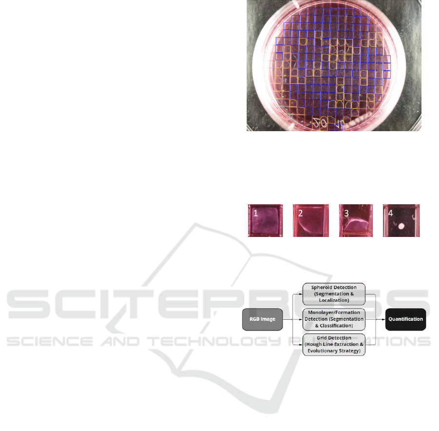
As shown in Figure 1, the datasets consist of petri dish

images from a digital single-lens reﬂex camera using

a 60mm F2.8 macro lens. All images provide a color

depth of 24 bits and a dimension of 4608 x 3456 pix-

els. All shown annotations are created using the slide

runner labeling tool (Aubreville et al., 2018)

Figure 1: Representation of an example image out of the

used dataset, including the manually labeled objects to be

segmented and classiﬁed. The blue marks represent the ini-

tial monolayer class. The yellow and gray marks are used

for the early and late formation of future spheroids. The

green color indicate the ﬁnal spheroids.

Figure 2: Example of the four stages from the initial mono-

layer (1) to the formation stages of early (2) and late (3)

formations until the ﬁnal spheroid form (4).

Figure 3: Simpliﬁed representation of the quantiﬁcation

workﬂow, including the three independent detection steps.

As shown by the individual cells in Figure 2, ini-

tially a monolayer (1) forms within each compartment

of the petri dish. During the ongoing formation pro-

cess, this monolayer transforms into the ﬁnal spheroid

form (4). The states in between are separated into

early (2) and late (3) formations, which are combined

into one formation class for the workﬂow in this pa-

per. The whole image dataset contains 20 images

which are divided into three separate sets for train-

ing the segmentation models (12 images), validation

(2 images) and testing (6 images).

2 METHODS

Our presented workﬂow has a modular design and is

based on three detection steps as shown in Figure 3.

This design decision allows future adjustments of the

used image processing algorithms as well as replace-

In Vitro Quantiﬁcation of Cellular Spheroids in Patterned Petri Dishes

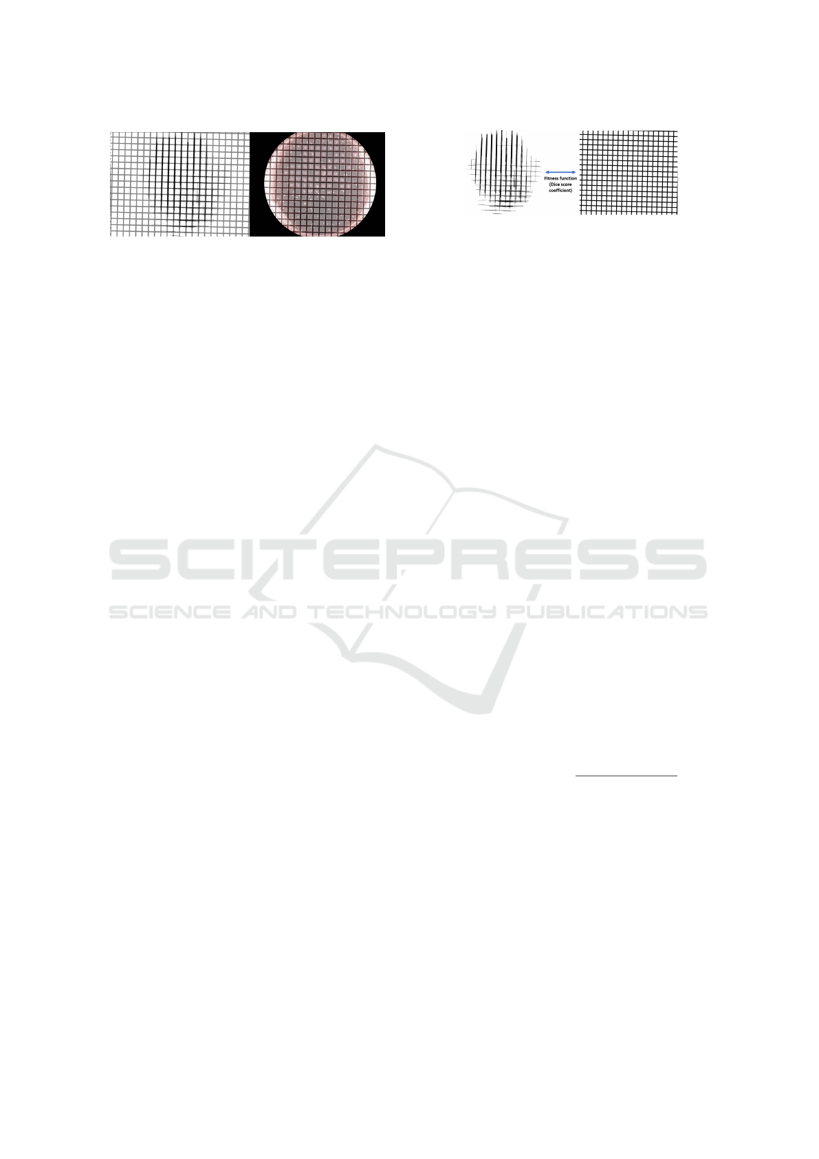
Figure 4: Examples of the grid identiﬁcation with the

mapped grid in binary (left) used for the ﬁtness function

and the mapped grid in the RGB image (right).

ments of the current segmentation neural networks.

2.1 Heuristic Grid Identiﬁcation

Grid mapping is performed to analyse single grid cells

in the image of a petri dish. A generated grid mask

maps the underlying grid. This grid mask deﬁnes sin-

gle grid cells and is used to extract the single grids

correctly. The grid is optimized with image process-

ing algorithms and an evolutionary strategy.

2.1.1 Preprocessing

Multiple preprocessing steps are performed before the

ﬁnal grid optimization can be executed. To avoid

possible noise outside of the petri dish and to fur-

ther on enable the identiﬁcation of grid cells within

it, the petri dish itself is extracted. This is achieved

by hough circles (Barabas et al., 2013; Forero et al.,

2020; Duda and Hart, 1972). The parameters for

blurring, canny edge detection, and the accumulator

threshold of the hough transformation were identiﬁed

manually on 14 images. It is presumed that the cen-

ter of the petri dish is within a window of 30% image

length in the middle of the image. As ﬁtness func-

tion of the evolutionary strategy, a binary mask is ex-

tracted automatically from the original RGB image.

This processed binary mask is used as a ground truth

image in the ﬁtness function, which is deﬁned by the

inverted Dice coefﬁcient, whereas the prediction is

the solution candidate representing a mask counting

a predicted grid (as shown in 5. To extract the binary

mask, after CLAHE, to increase the contrast, borders

are extracted with hough lines representing the grid

on the petri dish image (Zuiderveld, 1994; Duda and

Hart, 1972; Hansard et al., 2014). To allow the extrac-

tion of hough lines, a binary image with Roberts edge

detection is created based on the equalized RGB im-

age (Roberts et al., 1965; Bhardwaj and Mittal, 2012).

The connection of multiple extracted hough lines for

one line, is realized by morphological ﬁltering espe-

cially closing. Kernel size is reﬂected by the size

of the border and is extracted in relation to the im-

age size. The ﬁnal extracted mask, consists of white

Figure 5: Representative images for Dice coefﬁcient be-

tween preprocessing image used as ground truth (left) and

predicted grid (right).

background and black lines. A too-low minimum line

length increases the amount of noise within the image,

whereas a too high number of minimum line length

misses too many lines. In our evaluations, a mini-

mum length given with 10% of the image height pro-

vides robust results. In the experimental setup, light is

coming from the sides of the images, which increases

the contrast of vertical borders and allows an easier

extraction. Therefore, a lower threshold can be used

optionally for horizontal lines to avoid overlooking

them. With the described steps, a sufﬁcient amount

of horizontal and vertical borders are extracted within

the petri dish, which is important as ground truth for

a proper evaluation of the solution candidates.

2.1.2 Grid Optimization by Evolution strategy

Due to low contrast, shadows and disturbing effects,

not all borders in the image are visible or can be ex-

tracted from the image. Therefore, an evolution strat-

egy is used for the approximation of the full grid and

the prediction of missing borders in the petri dish

(Borgmann et al., 2012). The goal is to use the ex-

tracted lines in the preprocessing step as ground truth

and ﬁt a predicted full grid onto the extracted ground

truth image based on the ﬁtness function. The error of

the ﬁtness function is deﬁned by the Dice coefﬁcient

between the extracted binary images of the prepro-

cessing step containing the extracted lines and a pre-

dicted grid image represented by a solution candidate,

as shown in equation 1.

DiceC oe f f icient =

2 ∗ TP

2 ∗ T P + FP + FN

(1)

Deﬁned by: true positive (TP), false positive (FP) and

false negative (FN). Each solution candidate deﬁnes

a grid (see 6). Four adjustable parameters leaned on

afﬁne transformation parameters are used to represent

a grid:

• Rotation: Rotation of the grid lines to the origin.

• Scaling: Width of a single grid cell.

• Horizontal and Vertical offset: Position and trans-

lation of the grid.

For each solution candidate, an image containing the

grid using the parameters is created to evaluate the ﬁt-

ness of the solution candidate. An applicable amount

BIOIMAGING 2023 - 10th International Conference on Bioimaging

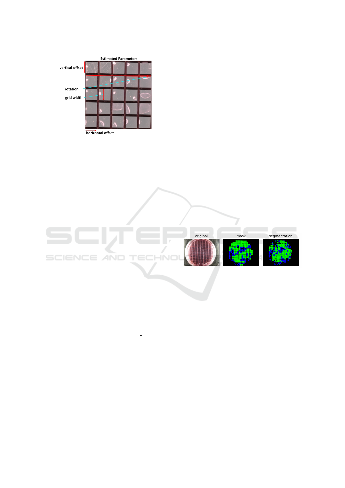
Figure 6: Explanation of solution candidate parameters.

for the population and starting sigma of the evolution-

ary strategy to allow a robust convergence was evalu-

ated. Elitism was used for the creation of new genera-

tions to keep the best candidate until this point. More-

over, the initial search space is reduced by problem-

speciﬁc constraints. The maximum width of a grid

cell also deﬁnes the maximum offset. Additionally,

the grid cells can not exceed 10% of the image’s

height. The rotation is limited to a maximum of 5

degrees. The evolutionary strategy is used for the op-

timization of the grid prediction and, therefore, the

accurate extraction of every single grid cell.

2.2 Object Detection

2.2.1 Segmentation Models

Descendent from the Unet architecture (Ronneberger

et al., 2015) which represents a specialized artiﬁ-

cial neural network for image segmentation, the used

Unet ++ (Zhou et al., 2018) represents the base ar-

chitecture for our segmentation models. Provided

by the segmentation models package (Iakubovskii,

2019) for the used Pytorch framework these models

were trained with the support of the Pytorch-lightning

framework (Falcon et al., 2019). Out of the several

provided backbones for the Unet ++ , our segmen-

tation models are built with the regnety 120 back-

bone (Radosavovic et al., 2020) which delivered the

best results for our use case. Due to limitations of

the available sample images, our modelling process

also included the use of data augmentation techniques

(Shorten and Khoshgoftaar, 2019) which represents

a commonly used approach for artiﬁcially extending

the available amount of image data. In our case, it

was necessary to use image cropping, which was re-

alised by randomly selecting small parts of the images

instead of using the whole image for the input of the

neural network. This technique was used on the train-

ing as well as the validation data. For the training

data, color and contrast adjustments combined with

image distortion, transposing, scaling, and rotation

added some variation in the available image proper-

ties. All in all, it was possible to extend our training

and validation data by a factor of 30. The separated

test data was not changed using any of the mentioned

algorithms. The original dataset without augmenta-

tion included 12 training images, 2 validation images

and 6 test images with a resolution of 4608x3456

pixel. The concept of using two models instead of

one is built up on the idea that the ﬁrst stages of a

forming spheroid can not move within the petri dish.

2.2.2 Monolayer and Forming Spheroids

Classiﬁcation

As Figure 7 shows, our segmentation model separates

the monolayers (blue) as well as the currently forming

spheroids (green) from the background represented

by the rest of the petri dish. This segmentation neu-

ral network classiﬁes the corresponding stage for each

pixel without the possibility for the same pixel to be

part of more than one class. This design decision was

made due to the property that these objects can not

overlay each other, which led to the use of a softmax

activation within the ﬁnal layer.

Figure 7: Example image of the segmentation result (right)

based on the raw RGB image (left) in comparison to the

mask (middle) representing the to be achieved separation

of the two classes. Green represents the already forming

spheroids out of the blue monolayer.

To further improve the accuracy of the prediction

used for a ﬁnal quantiﬁcation of monolayer cells and

currently forming spheroid cells, a prediction for ev-

ery single grid cell is performed. The prediction is

based on the segmentation results. Since a predic-

tion of both classes can be within a single grid cell

of the grid a ﬁnal decision to correctly classify such a

grid cell has to be made. The quantiﬁcation of each

cell type is allowed by the assignment of the class to

each valid grid cell. Only grid cells within the petri

dish are considered. Therefore, grid cells that are not

fully within the petri dish and grid cells with a high

percentage of background are removed for the eval-

uation since they cannot contain any cell or the cell

is cut and not fully in the image. The estimated grid

deﬁnes each grid cell. For each grid cell, a predic-

tion of either one class is performed. If a grid cell

In Vitro Quantiﬁcation of Cellular Spheroids in Patterned Petri Dishes

contains a prediction for a monolayer, it is assigned

as a monolayer and vice versa for the second class of

forming spheroids. A prediction within a grid cell is

extracted by connected components. If both classes

are predicted within a single grid cell, the monolayer

class is taken if the predicted overall area is larger or

if the conﬁdence of the model is higher in comparison

to the second class. This is suitable since monolayers

are larger by deﬁnition.

2.2.3 Spheroid Localization

In contrast to the monolayer and forming spheroid

stages, the ﬁnal spheroid objects can move around and

overlay other objects. This property could lead to a

pixel with more than one class, which is possible by

using a second model speciﬁcally for this class. Nor-

mally, this would be realized by a multiclass segmen-

tation model for all stages at once, but this decision

would inhibit the ability of the workﬂow to only allow

spheroid objects to overlap other classes. As shown in

Figure 8: Example of the test dataset with an overlay of

the segmentation on the original RGB image. All detected

spheroids are represented by the white dots.

Figure 8 this second neural network only separates the

possible spheroid objects from the background with-

out any knowledge of the other stages. Therefore,

all the other stages are considered as background.

Based on this segmentation result, the actual local-

ization of the individual objects is realized using the

connected components algorithm from the Open CV

Python framework (OpenCV, 2015). After a ﬁltering

step that removes every object smaller than 70 percent

of the average object size, the resulting objects are lo-

cated by their center pixel as assigned to the spheroid

class for the ﬁnal quantiﬁcation step. This size ﬁlter-

ing has to be done individually for each image to be

segmented by the fact that the object size also relies

on the camera parameters and the used lens. There-

fore, it would not be possible to set a speciﬁc size limit

for all now-arriving objects. This 70 percent of the av-

erage size limit was set based on the current dataset.

It still allows some wrong detected objects, but it in-

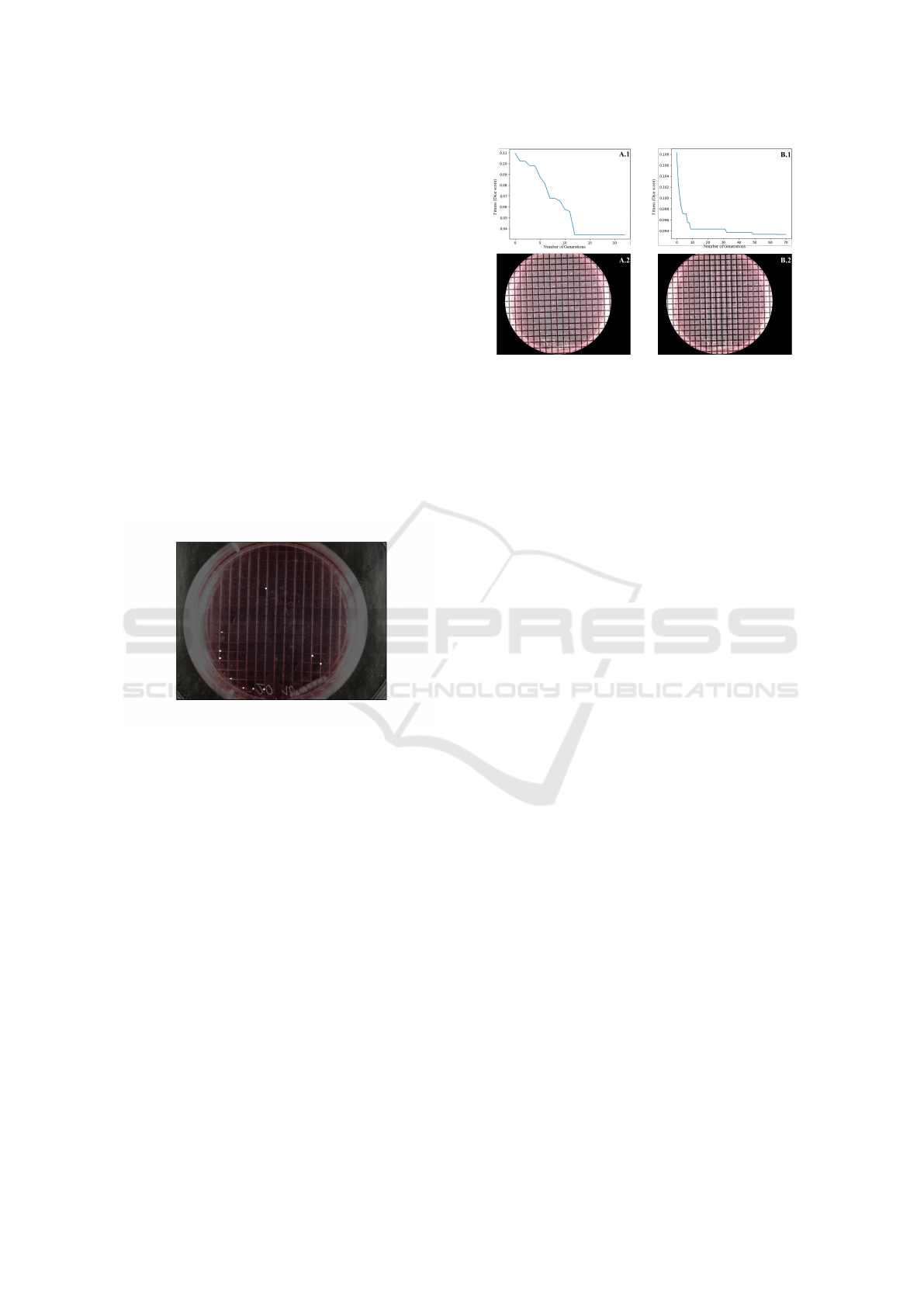
Figure 9: Comparison of a sufﬁcient and insufﬁcient result

for grid alignment on an image of a petri dish.

hibits nearly all artifacts that are smaller than all valid

spheroids, like wrongly as spheroids detected reﬂec-

tions or air bubbles. Based on the used imaging setup,

this limit can be adjusted by the user for future appli-

cations. Due to the possibility of the ﬁnal spheroid

stage merging together with other spheroids, an up-

per size limit is not considered to have any positive

impact on the segmentation quality.

3 RESULTS

3.1 Monolayer & Forming Spheroid

Quantiﬁcation

3.1.1 Parameter evaluation of Grid Estimation

In Figure 9 the applicability of the evolutionary strat-

egy and its used ﬁtness function is shown. Two differ-

ent results on the same image with its corresponding

ﬁtness score histories can be seen. In the ﬁrst results

(A.1 and A.2) the ﬁtness is improved over multiple

generations down to a value of 0.034. The low value

is also connected to a good result (as shown in sub-

image A.2). Whereas in the second result (B.1 and

B.2) the error (ﬁtness score) can be reduced slightly

in the ﬁrst generations but there is no further improve-

ment also after multiple generations. This states a

false optimization in a local optimum and is reﬂected

in a higher value of 0.093. The higher error is also re-

ﬂected in the corresponding sub-image (B.2), as it can

clearly be seen that the grid is not aligned and even

divides the actual grid cells on the petri dish into two

parts. The second result was generated by an ES with

an insufﬁcient size for the population. The aligned

grid and the converging error over multiple genera-

tions in sub-images A.1 and A.2 show the applicabil-

ity of the used ﬁtness function and also the overall

approach.

BIOIMAGING 2023 - 10th International Conference on Bioimaging

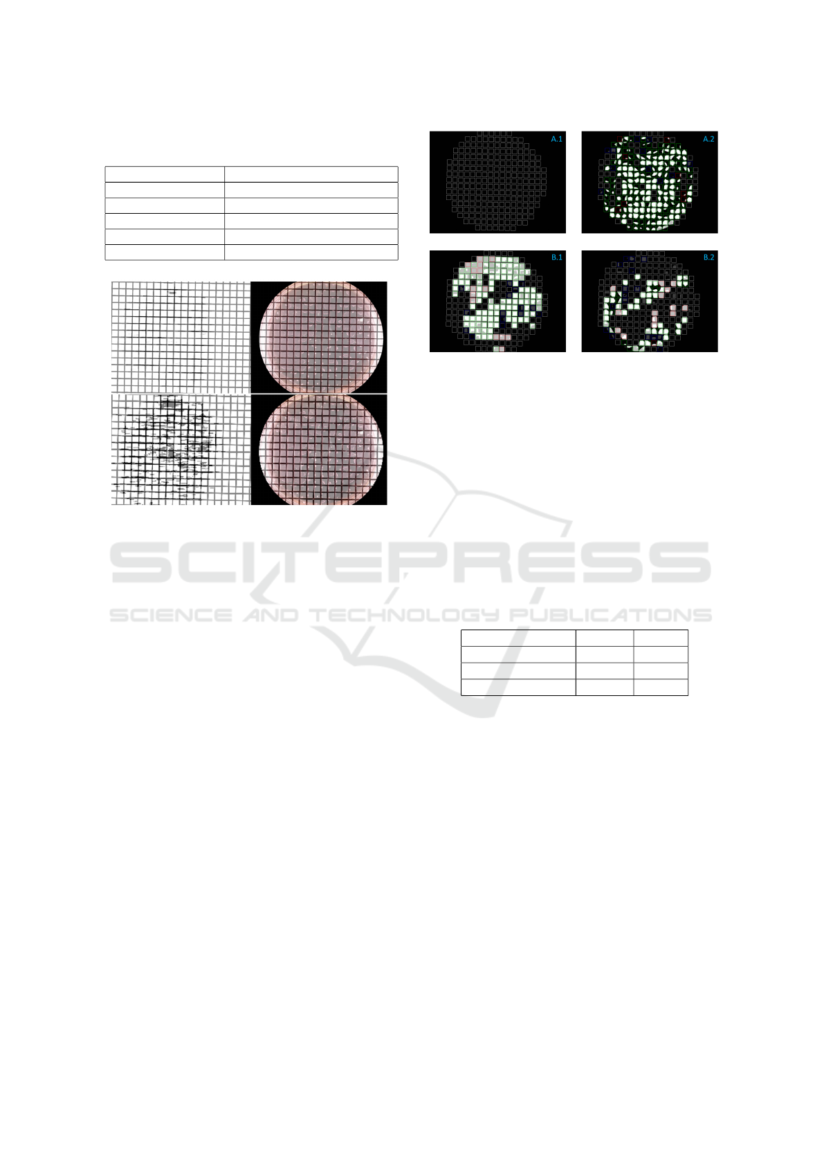
Table 1: Fitness comparison of multiple runs with different

settings for the evolutionary strategy.

Population sigma mean ± std [min - max]

1,50 0.05 0.086 ± 0.003 [0.063 - 0.229]

10,50 0.05 0.063 ± 0.005 [0.052 - 0.229]

20,100 0.05 0.061 ± 0.005 [0.05 - 0.231]

20,100 0.1 0.062 ± 0.01 [0.048 - 0.229]

20,100 0.001 0.125 ± 0.048 [ 0.044 - 0.25]

Figure 10: Example results of the mapped grid on an image

with different resolutions (row 1: factor 1.25, row 3: Factor

0.25). On the left the overlap of the grid and the binary

image can be seen. on the right the ﬁtted grid on the rgb

images is shown.

As shown in Table 1, multiple runs for a differ-

ent setting for the population of the ES and the ini-

tial sigma were performed. In it, the average error

over 20 images is shown. The used setting with 20

parents and 100 children and an initial sigma of 0.05

provides the best and most robust results with the low-

est average error of 0.061 and a standard deviation

of 0.005. Whereas other runs with a higher starting

sigma (0.01) and a lower amount for the population

(10,50) provide similar results, lower values for the

population, especially with only one parent or a lower

starting value of sigma for faster convergence is in-

sufﬁcient and provides clearly worse results reﬂected

in a higher error of 0.086 and 0.125.

As it is important that the grid detection also

works size independently, example images of differ-

ent sizes can be seen in Figure 10. The shown res-

olutions are factor 1.25 and 0.25. In a both results

(rows) the grid is aligned correctly. For resize fac-

tor 1.25 in all tested images, the grid was identiﬁed

correctly. The grid lies perfectly on the preprocessed

image. The preprocessed image also contains a very

low amount of noise and a large amount of extracted

hough lines. With smaller images, the amount of

noise increases. The result in row 2 shows a worst

Figure 11: Final grid cell prediction based on two example

images (A and B) for the prediction results of both classes

(monolayer and starting formation). The Figure shows the

ﬁnal evaluation of the algorithm with its assignments per

grid cell (white: true negative, green: true positive, blue:

false positive, red: false negative).

case scenario with a high amount of noise, but still

shows a correct gird. In almost all cases, the evo-

lutionary strategy is robust enough to allow a cor-

rect alignment also in smaller images or images with

higher noise.

3.1.2 Segmentation of Monolayer & Starting

Formation

Table 2: Monolayer and forming spheroids segmentation

quality measurements on the test dataset.

Class Jaccard F1

Empty 0.8739 0.9671

Monolayer 0.5995 0.3674

Forming spheroid 0.7969 0.7754

As shown in Table 2, our segmentation neural net-

work can identify empty cells and already forming

spheroids with an F1 score of over 0.9671 for the

empty ones and a slightly lower score of 0.7754 for

the forming spheroid class. The main struggle for our

network is the identiﬁcation of the monolayer class,

which led us to the presented post-processing steps

for an increase of the initial F1 score as low as 0.3674.

3.1.3 Classiﬁcation Monolayer and Starting

Formation

In the ﬁnal object detection step the quantiﬁcation for

each relevant type of cell is fulﬁlled. In Figure 11 the

classiﬁcation and quantiﬁcation of monolayers (class

1) and starting formation cells (class 2) can is shown.

In the ﬁgure the results for both classes on two exam-

ple images are shown (Image A, and Image B). Image

In Vitro Quantiﬁcation of Cellular Spheroids in Patterned Petri Dishes

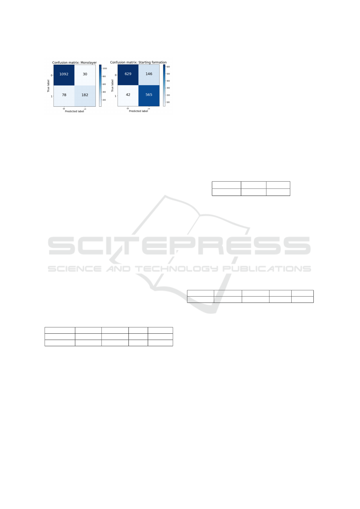
Figure 12: Confusion matrix of grid cell classiﬁcation for

the classes monolayer & starting formation).

A shows a result without any monolayer cells in the

ground truth. The predictions for the monolayer class

in sub-image A.1 are all correctly true negative. The

model can therefore predict correctly even if there is

no cell in that class. In the prediction of the monolay-

ers (image B.1) in image B a high amount of mono-

layers can be seen. It can be seen that the models’

prediction and the subsequent class assignment to a

grid cell do indicate good results. Despite some false

positives (blue colored grid cells) and false negatives

(red colored grid cells) the prediction result can be

considered as good. Most errors in class 1 appear in

monolayer cells that span the whole grid cell with bad

lighting or starting formations cells that just started

and are still covering almost a full grid cell. Another

problem is the mentioned division of a single cell into

two different classes, which can lead to false nega-

tives in one class and false positives in the other cells.

These problems can also be seen in sub-images B.1

and B2, where most false negatives are starting for-

mation cells with almost full coverage of the grid cell.

In sub-image A.2 these problems appear much less

therefore, a higher performance can be reached. All

in all, the approach shows minor problems with bor-

der cases but a good overall performance.

Table 3: Metrics of grid cell classiﬁcation for the classes

monolayer and starting formation.

class accuracy precision recall f1-score

monolayer 0.92 0.86 0.70 0.77

formation 0.86 0.80 0.93 0.86

The general performance on all test images is

shown in Table 3 and Figure 12. The result shows a

high accuracy of 0.92 for class 1 and 0.86 for class 2.

Especially the predictions for the monolayer cells do

have high accuracy. This is in comparison to the class

with cells that started the formation due to a very good

prediction of true negatives (also shown in sub-image

A.1 in Figure 11). Overall, the prediction of cells with

starting formation provides slightly better results, as

shown in the f1-score. With scores of 0.77 and 0.86

the error, especially for cells of the starting forma-

tion class, is low. The lower f1-score in the ﬁrst class

can be explained by a lower recall resulting in more

missed cells, whereas the precision is higher. For the

class of starting formations, most cells are detected

with slightly lower precision. Both have a consider-

ably high performance. With a f1-score of 0.77 and

0.86, the ﬁnal quantiﬁcation was increased in com-

parison to the performance of the segmentation itself

and subsequently allows a good automatized quantiﬁ-

cation.

3.2 Spheroid localisation

As shown in Table 4, the raw segmentation mask can

not provide the demanded quality for accurate quan-

tiﬁcation of the spheroids within an image.

Table 4: Spheroids segmentation quality measured on the

test dataset.

Class Jaccard F1

Spheroid 0.7642 0.6889

The exceptionally low F1/Dice Score is signiﬁ-

cantly increased during the post-processing, including

the actual location of the ﬂoating objects, as shown

in Table 5. As explained in section 2.2.3, the local-

ization of each spheroid is represented by its center

pixel. Based on these coordinates, the quality mea-

sures of Table 5 where realized by the comparison

with the label masks. The mentioned ﬁltering, as well

as the added localisation workﬂow increased the ﬁnal

F1 Score from 0.6889 to 0.8457.

Table 5: Spheroids localisation quality measured on the test

dataset.

Class Accuracy Precision Recall F1

Spheroid 0.7327 0.8962 0.8007 0.8457

As shown in the confusion matrix of Figure 13,

most of the actual spheroid objects are segmented

and classiﬁed correctly. Despite the high amount of

falsely as background detected objects, the number of

false positives could be kept on a signiﬁcantly lower

level, which is realized by the mentioned size ﬁlter.

Without this ﬁlter, the number of false positives would

increase signiﬁcantly by a factor of 6.5 due to the in-

creased amount of noise detected as objects.

4 DISCUSSION AND OUTLOOK

Regarding the presented results, our workﬂow already

provides the functionality for the automated quantiﬁ-

cation of cell compartments on petri dishes by form-

ing spheroids based on RGB images. Simply im-

aged using a normal DSLR camera, these images are

BIOIMAGING 2023 - 10th International Conference on Bioimaging

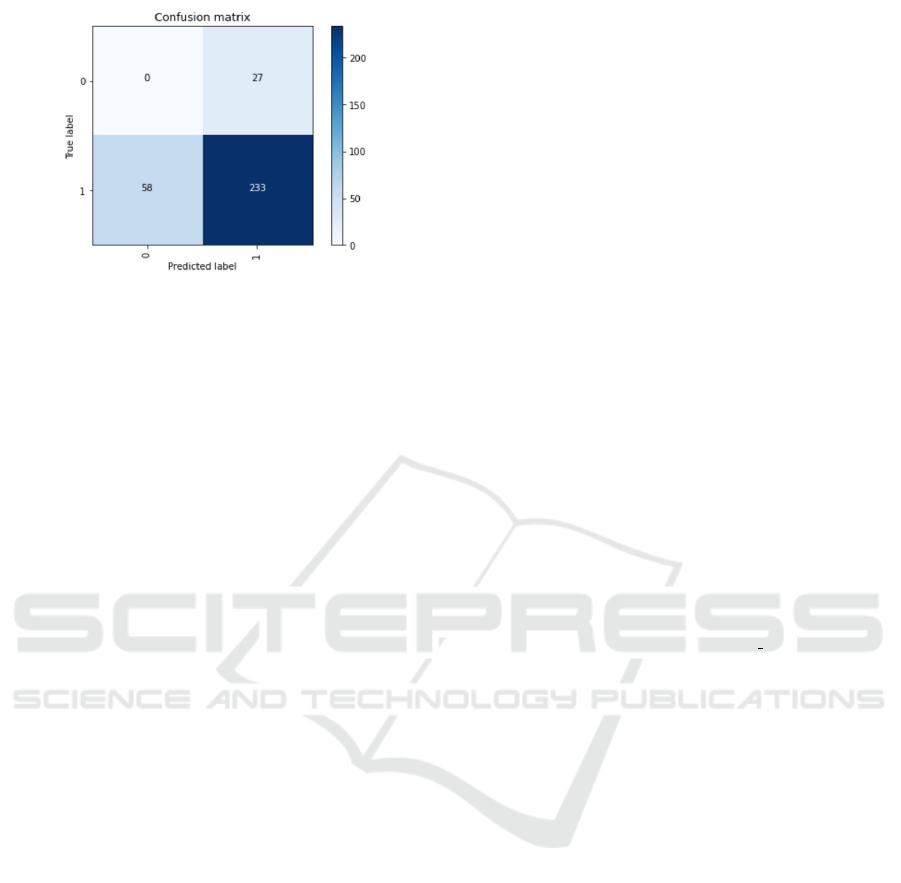
Figure 13: Confusion matrix of the spheroid localisation

showing result measures on the test dataset.

processed using a combination of machine learning

algorithms, heuristic optimization, and computer vi-

sion. This combination of state-of-the-art algorithms

allows our workﬂow to quantify different stages of

forming spheroids which will be used for statistical

analysis in future work, including the inﬂuence of dif-

ferent drugs measured over a period of time. De-

spite the low initial segmentation quality, our pre-

sented post-processing and quantiﬁcation algorithms

increases the classiﬁcation performance of our work-

ﬂow signiﬁcantly, which still allows reliable quan-

tiﬁcation of the different stages. In future different

segmentation methods will be further evaluated to in-

crease the overall performance. Regarding these ﬁrst

results, the amount of data used for the modeling steps

will be increased signiﬁcantly in future work, which

should further increase the ﬁnal quality of the quan-

tiﬁcation.

ACKNOWLEDGEMENTS

This work was supported by the Center of Excellence

for Technical Innovation in Medicine (TIMed), the

Dissertation Programme of the University of Applied

Sciences Upper Austria and the Austrian Research

Promotion Agency (FFG, project no. 881547 and In-

dustrienahe Dissertation no 867720).

REFERENCES

Aubreville, M., Bertram, C., Klopﬂeisch, R., and Maier, A.

(2018). SlideRunner - A Tool for Massive Cell An-

notations in Whole Slide Images. In Bildverarbeitung

ur die Medizin 2018, pages 309–314. Springer Berlin

Heidelberg.

Barabas, J., Radil, R., and Gombarska, D. (2013). Image

processing and feature extraction of circular objects

from biological images. In 2013 36th International

Conference on Telecommunications and Signal Pro-

cessing (TSP), pages 612–615. IEEE.

Bhardwaj, S. and Mittal, A. (2012). A survey on vari-

ous edge detector techniques. Procedia Technology,

4:220–226.

Borgmann, D., Weghuber, J., Schaller, S., Jacak, J., and

Winkler, S. (2012). Identiﬁcation of patterns in mi-

croscopy images of biological samples using evolu-

tion strategies. In Proceedings of the 24th European

Modeling and Simulation Symposium, pages 19–21.

Duda, R. O. and Hart, P. E. (1972). Use of the hough trans-

formation to detect lines and curves in pictures. Com-

munications of the ACM, 15(1):11–15.

Falcon, W. et al. (2019). Pytorch lightning. GitHub.

Note: https://github.com/PyTorchLightning/pytorch-

lightning, 3(6).

Forero, M. G., Medina, L. A., Hern

andez, N. C., and Mor-

era, C. M. (2020). Evaluation of the hough and ransac

methods for the detection of circles in biological tests.

In Applications of Digital Image Processing XLIII,

volume 11510, pages 387–395. SPIE.

ursatz, M., Gerges, P., Wolbank, S., and N

urnberger,

S. (2021). Autonomous spheroid formation by

culture plate compartmentation. Biofabrication,

13(3):035018.

Hansard, M., Horaud, R., Amat, M., and Evangelidis, G.

(2014). Automatic detection of calibration grids in

time-of-ﬂight images. Computer Vision and Image

Understanding, 121:108–118.

Iakubovskii, P. (2019). Segmentation models pytorch. https:

//github.com/qubvel/segmentation models.pytorch.

Johnstone, B., Hering, T. M., Caplan, A. I., Goldberg,

V. M., and Yoo, J. U. (1998). In vitrochondrogene-

sis of bone marrow-derived mesenchymal progenitor

cells. Experimental cell research, 238(1):265–272.

OpenCV (2015). Open source computer vision library.

Radosavovic, I., Kosaraju, R. P., Girshick, R., He, K., and

Doll

ar, P. (2020). Designing network design spaces.

Roberts, L. et al. (1965). Machine perception of three-

dimensional solids, optical and electro-optical infor-

mation processing. MIT Press, Cambridge, MA, pages

159–197.

Ronneberger, O., Fischer, P., and Brox, T. (2015). U-net:

Convolutional networks for biomedical image seg-

mentation. In Lecture Notes in Computer Science.

Shorten, C. and Khoshgoftaar, T. M. (2019). A survey on

image data augmentation for deep learning. Journal

of Big Data, 6:60.

Zhang, L., Su, P., Xu, C., Yang, J., Yu, W., and Huang, D.

(2010). Chondrogenic differentiation of human mes-

enchymal stem cells: a comparison between micro-

mass and pellet culture systems. Biotechnology let-

ters, 32(9):1339–1346.

Zhou, Z., Siddiquee, M. M. R., Tajbakhsh, N., and Liang,

J. (2018). Unet++: A nested u-net architecture for

medical image segmentation. volume 11045 LNCS.

Zuiderveld, K. (1994). Contrast limited adaptive histogram

equalization. Graphics gems, pages 474–485.

In Vitro Quantiﬁcation of Cellular Spheroids in Patterned Petri Dishes